Recognizing users' physical activity with examples on R
The problem of recognizing the physical activity of users (Human activity Recognition or HAR) came across to me earlier only as training tasks. Having discovered the possibilities of the Caret R Package , a convenient wrapper for over 100 machine learning algorithms, I decided to try it for HAR. The UCI Machine Learning Repository has several data sets for such experiments. Since the topic with dumbbells for me is not very close, I chose to recognize the activity of smartphone users .
The data in the set was obtained from thirty volunteers with Samsung Galaxy S II attached to the belt. The signals from the gyroscope and accelerometer were specially processed and transformed into 561 signs. For this, multistage filtering, Fourier transform and some standard statistical transformations were used, 17 functions altogether: from the mathematical expectation to the calculation of the angle between the vectors. I’m missing the details of processing, they can be found in the repository. The training sample contains 7352 cases, the test sample contains 2947. Both samples are marked with tags corresponding to six activities: walking, walking_up, walking_down, sitting, standing and laying.
As a basic algorithm for experiments, I chose Random Forest. The choice was based on the fact that RF has a built-in mechanism for assessing the importance of variables, which I wanted to experience, since the prospect of self-selection of signs from the 561 variable scared me a little. I also decided to try the support vector machine (SVM). I know that this is a classic, but I didn’t have to use it before, it was interesting to compare the quality of the models for both algorithms.
Having downloaded and unpacked the archive with the data, I realized that I would have to tinker with it. All parts of the set, the names of signs, activity labels were in different files. To upload files to R, I used the read.table () function. It was necessary to prohibit the automatic conversion of rows into factor variables, as it turned out that there are duplicate variable names. In addition, the names contained incorrect characters. This problem was solved by the following construction with the sapply () function, which in R often replaces the standard for loop:
')
I stuck all the parts of the sets using the rbind () and cbind () functions. The first connects the rows of the same structure, the second column of the same length.
After I prepared a training and test sample, the question arose about the need for data preprocessing. Using the range () function in a loop, calculated a range of values. It turned out that all signs are within [-1,1] and it means that neither normalization nor scaling is necessary. Then I checked for signs with a highly biased distribution. For this, I used the skewness () function from the e1071 package:
Apply () is a function from the same category as sapply () , used when something needs to be done in columns or rows. train_data [, - 1] - a data set without a dependent variable Activity, 2 indicates that it is necessary to calculate the value by columns. This code prints the three worst variables:
The closer these values are to zero, the less is the distortion of the distribution, and here it is, frankly, rather big. In this case, caret has a BoxCox transformation implementation. I read that Random Forest is not sensitive to such things, so I decided to leave the signs as they are and at the same time to see how the SVM will cope with this.
It remains to choose the model quality criterion: Accuracy accuracy or accuracy or Kappa acceptance criterion. If the cases of classes are unevenly distributed, you need to use Kappa, this is the same Accuracy only taking into account the probability to randomly “pull out” one or another class. By making summary () for the Activity column, checked the distribution:
Cases are distributed almost equally, except maybe walking_down (some of the volunteers apparently did not really like to go down the stairs), which means you can use Accuracy.
Trained RF model on the full set of features. For this, the following construction on R was used:
It provides k-fold cross-validation with k = 5. By default, three models are trained with different mtry values (the number of signs that are randomly selected from the entire set and are considered as a candidate for each branching tree), and then the best one is selected by accuracy. The number of trees for all models is the same ntree = 100.
To determine the quality of the model on the test sample, I took the confusionMatrix (x, y) function from caret, where x is the vector of predicted values, and y is the vector of values from the test sample. Here is part of her issue:
Training on the full set of features took about 18 minutes on a laptop with an Intel Core i5. It could have been done several times faster on OS X, using several processor cores using the doMC package, but for Windows there is no such thing, as far as I know.
Caret supports several SVM implementations. I chose svmRadial (SVM with a core - a radial basis function), it is often used with caret, and is a general tool when there is no special information about the data. To train a model with SVM, simply change the value of the method parameter in the train () function to svmRadial and remove the do.trace and ntree parameters. The algorithm showed the following results: Accuracy on the test sample - 0.952. In this case, the training of the model with five-fold cross-validation took a little more than 7 minutes. Left a note on the memory: do not grab immediately for the Random Forest.
You can get the results of the built-in assessment of the importance of variables in RF using the varImp () function from the caret package. The construction of the plot view (varImp (model), 20) will reflect the relative importance of the first 20 signs:

"Acc" in the title indicates that this variable was obtained by processing the signal from the accelerometer, "Gyro", respectively, from the gyroscope. If you look closely at the graph, you can make sure that there are no data from the gyroscope among the most important variables, which is surprising and inexplicable for me personally. (“Body” and “Gravity” are two components of the signal from the accelerometer, t and f are the time and frequency domains of the signal).
Substituting in RF attributes, selected by importance, meaningless exercise, he had already selected and used them. But with the SVM can happen. I started with 10% of the most important variables and began to increase by 10% each time controlling the accuracy, finding the maximum, reduced the step first to 5%, then to 2.5%, and finally to one variable. The result - the maximum of accuracy was in the area of 490 signs and amounted to 0.9545, which is better than the value on the full set of signs by only a quarter percent (an extra pair of correctly classified cases). This work could be automated, as part of the caret is the implementation of RFE (Recursive feature elimination), it recursively removes and adds one variable each and controls the accuracy of the model. There are two problems with it, RFE works very slowly (inside Random Forest), for a data set that is similar in number of features and cases, the process would take about a day. The second problem is the accuracy on the training sample, which RFE evaluates, it is not at all the same as the accuracy on the test sample.
The code that extracts from varImp and orders, in descending order of importance, the names of a given number of attributes, looks like this:
To clear my conscience, I decided to try some other method of selecting signs. I chose to filter features based on the calculation of the information gain ratio (it is found as an information gain or information gain), a synonym for Kullback-Leibler divergence. IGR is a measure of the differences between the probability distributions of two random variables.
To calculate IGR, I used the information.gain () function from the FSelector package. The package needs a JRE to work. Incidentally, there are other tools that allow you to select features based on entropy and correlation. The IGR values are inverse to the “distance” between the distributions and normalized [0.1], i.e. the closer to one the better. After calculating the IGR, I ordered the list of variables in descending order of IGR, the first 20 looked like this:
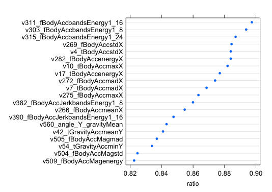
IGR gives a completely different set of "important" signs, with important only five coincided. There is no gyroscope in the top again, but there are a lot of signs with the X component. The maximum IGR value is 0.897, the minimum is 0. After receiving an ordered list of features, it acted with it as well as with importance. Checked on SVM and RF, significantly increase the accuracy did not work.
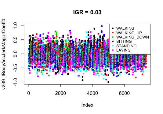
I think that the selection of signs in similar tasks does not always work, and there are at least two reasons. The first reason is related to the construction of features. The researchers, who prepared the data set, tried to "survive" all the information from the signals from the sensors and did it for sure consciously. Some signs give more information, some less (only one variable turned out to be zero with an IGR). This is clearly seen if you plot graphs of the values of attributes with different IGR levels. For definiteness, I chose the 10th and 551st. It is seen that for a sign with a high IGR, the points are well visually separable, with a low IGR - they resemble a color mixture, but obviously they carry some piece of useful information.

The second reason is related to the fact that the dependent variable is a factor with more than two levels (here - six). Reaching maximum accuracy in one class, we deteriorate in the other. This can be shown on the mismatch matrices for two different sets of features with the same accuracy:
In the upper variant, there are fewer errors in the first two classes, in the lower variant, in the third and fifth.
Summing up:
1. SVM “made” Random Forest in my task, works twice as fast and gives a better model.
2. It would be correct to understand the physical meaning of variables. And, it seems, on a gyroscope in some devices you can save.
3. The importance of variables from RF can be used to select variables with other teaching methods.
4. Selection of features based on filtering does not always improve the quality of the model, but at the same time reduces the number of features, reducing training time with a slight loss in quality (when using 20% of important variables, the accuracy in SVM was only 3% lower than the maximum).
The code for this article can be found in my repository .
A few additional links:
UPD:
On the advice of kenoma , a major component analysis (PCA) was done. Used a variant with the caret preProcess function:
A cutoff of 0.95, it turned out 102 components.
RF accuracy on the test sample: 0.8734 (5% lower than accuracy on the full set)
SVM accuracy: 0.9386 (one percent lower). I think this result is quite good, so the advice was useful.
Data
The data in the set was obtained from thirty volunteers with Samsung Galaxy S II attached to the belt. The signals from the gyroscope and accelerometer were specially processed and transformed into 561 signs. For this, multistage filtering, Fourier transform and some standard statistical transformations were used, 17 functions altogether: from the mathematical expectation to the calculation of the angle between the vectors. I’m missing the details of processing, they can be found in the repository. The training sample contains 7352 cases, the test sample contains 2947. Both samples are marked with tags corresponding to six activities: walking, walking_up, walking_down, sitting, standing and laying.
As a basic algorithm for experiments, I chose Random Forest. The choice was based on the fact that RF has a built-in mechanism for assessing the importance of variables, which I wanted to experience, since the prospect of self-selection of signs from the 561 variable scared me a little. I also decided to try the support vector machine (SVM). I know that this is a classic, but I didn’t have to use it before, it was interesting to compare the quality of the models for both algorithms.
Having downloaded and unpacked the archive with the data, I realized that I would have to tinker with it. All parts of the set, the names of signs, activity labels were in different files. To upload files to R, I used the read.table () function. It was necessary to prohibit the automatic conversion of rows into factor variables, as it turned out that there are duplicate variable names. In addition, the names contained incorrect characters. This problem was solved by the following construction with the sapply () function, which in R often replaces the standard for loop:
')
editNames <- function(x) { y <- var_names[x,2] y <- sub("BodyBody", "Body", y) y <- gsub("-", "", y) y <- gsub(",", "_", y) y <- paste0("v",var_names[x,1], "_",y) return(y) } new_names <- sapply(1:nrow(var_names), editNames) I stuck all the parts of the sets using the rbind () and cbind () functions. The first connects the rows of the same structure, the second column of the same length.
After I prepared a training and test sample, the question arose about the need for data preprocessing. Using the range () function in a loop, calculated a range of values. It turned out that all signs are within [-1,1] and it means that neither normalization nor scaling is necessary. Then I checked for signs with a highly biased distribution. For this, I used the skewness () function from the e1071 package:
SkewValues <- apply(train_data[,-1], 2, skewness) head(SkewValues[order(abs(SkewValues),decreasing = TRUE)],3) Apply () is a function from the same category as sapply () , used when something needs to be done in columns or rows. train_data [, - 1] - a data set without a dependent variable Activity, 2 indicates that it is necessary to calculate the value by columns. This code prints the three worst variables:
 v389_fBodyAccJerkbandsEnergy57_64 v479_fBodyGyrobandsEnergy33_40 v60_tGravityAcciqrX
 14.70005 12.33718 12.18477
The closer these values are to zero, the less is the distortion of the distribution, and here it is, frankly, rather big. In this case, caret has a BoxCox transformation implementation. I read that Random Forest is not sensitive to such things, so I decided to leave the signs as they are and at the same time to see how the SVM will cope with this.
It remains to choose the model quality criterion: Accuracy accuracy or accuracy or Kappa acceptance criterion. If the cases of classes are unevenly distributed, you need to use Kappa, this is the same Accuracy only taking into account the probability to randomly “pull out” one or another class. By making summary () for the Activity column, checked the distribution:
      WALKING WALKING_UP WALKING_DOWN SITTING STANDING LAYING
         1226 1073 986 1286 1374 1407
Cases are distributed almost equally, except maybe walking_down (some of the volunteers apparently did not really like to go down the stairs), which means you can use Accuracy.
Training
Trained RF model on the full set of features. For this, the following construction on R was used:
fitControl <- trainControl(method="cv", number=5) set.seed(123) forest_full <- train(Activity~., data=train_data, method="rf", do.trace=10, ntree=100, trControl = fitControl) It provides k-fold cross-validation with k = 5. By default, three models are trained with different mtry values (the number of signs that are randomly selected from the entire set and are considered as a candidate for each branching tree), and then the best one is selected by accuracy. The number of trees for all models is the same ntree = 100.
To determine the quality of the model on the test sample, I took the confusionMatrix (x, y) function from caret, where x is the vector of predicted values, and y is the vector of values from the test sample. Here is part of her issue:
               Reference
 Prediction WALKING WALKING_UP WALKING_DOWN SITTING STANDING LAYING
   WALKING 482 38 17 0 0 0
   WALKING_UP 7,426 37 0 0 0
   WALKING_DOWN 7 7 366 0 0 0
   SITTING 0 0 0 433 51 0
   STANDING 0 0 0 58 481 0
   LAYING 0 0 0 0 0 537
 Overall Statistics
                Accuracy: 0.9247
                  95% CI: (0.9145, 0.9339)
Training on the full set of features took about 18 minutes on a laptop with an Intel Core i5. It could have been done several times faster on OS X, using several processor cores using the doMC package, but for Windows there is no such thing, as far as I know.
Caret supports several SVM implementations. I chose svmRadial (SVM with a core - a radial basis function), it is often used with caret, and is a general tool when there is no special information about the data. To train a model with SVM, simply change the value of the method parameter in the train () function to svmRadial and remove the do.trace and ntree parameters. The algorithm showed the following results: Accuracy on the test sample - 0.952. In this case, the training of the model with five-fold cross-validation took a little more than 7 minutes. Left a note on the memory: do not grab immediately for the Random Forest.
Importance of variables
You can get the results of the built-in assessment of the importance of variables in RF using the varImp () function from the caret package. The construction of the plot view (varImp (model), 20) will reflect the relative importance of the first 20 signs:

"Acc" in the title indicates that this variable was obtained by processing the signal from the accelerometer, "Gyro", respectively, from the gyroscope. If you look closely at the graph, you can make sure that there are no data from the gyroscope among the most important variables, which is surprising and inexplicable for me personally. (“Body” and “Gravity” are two components of the signal from the accelerometer, t and f are the time and frequency domains of the signal).
Substituting in RF attributes, selected by importance, meaningless exercise, he had already selected and used them. But with the SVM can happen. I started with 10% of the most important variables and began to increase by 10% each time controlling the accuracy, finding the maximum, reduced the step first to 5%, then to 2.5%, and finally to one variable. The result - the maximum of accuracy was in the area of 490 signs and amounted to 0.9545, which is better than the value on the full set of signs by only a quarter percent (an extra pair of correctly classified cases). This work could be automated, as part of the caret is the implementation of RFE (Recursive feature elimination), it recursively removes and adds one variable each and controls the accuracy of the model. There are two problems with it, RFE works very slowly (inside Random Forest), for a data set that is similar in number of features and cases, the process would take about a day. The second problem is the accuracy on the training sample, which RFE evaluates, it is not at all the same as the accuracy on the test sample.
The code that extracts from varImp and orders, in descending order of importance, the names of a given number of attributes, looks like this:
imp <- varImp(model)[[1]] vars <- rownames(imp)[order(imp$Overall, decreasing=TRUE)][1:56] Feature filtering
To clear my conscience, I decided to try some other method of selecting signs. I chose to filter features based on the calculation of the information gain ratio (it is found as an information gain or information gain), a synonym for Kullback-Leibler divergence. IGR is a measure of the differences between the probability distributions of two random variables.
To calculate IGR, I used the information.gain () function from the FSelector package. The package needs a JRE to work. Incidentally, there are other tools that allow you to select features based on entropy and correlation. The IGR values are inverse to the “distance” between the distributions and normalized [0.1], i.e. the closer to one the better. After calculating the IGR, I ordered the list of variables in descending order of IGR, the first 20 looked like this:

IGR gives a completely different set of "important" signs, with important only five coincided. There is no gyroscope in the top again, but there are a lot of signs with the X component. The maximum IGR value is 0.897, the minimum is 0. After receiving an ordered list of features, it acted with it as well as with importance. Checked on SVM and RF, significantly increase the accuracy did not work.
I think that the selection of signs in similar tasks does not always work, and there are at least two reasons. The first reason is related to the construction of features. The researchers, who prepared the data set, tried to "survive" all the information from the signals from the sensors and did it for sure consciously. Some signs give more information, some less (only one variable turned out to be zero with an IGR). This is clearly seen if you plot graphs of the values of attributes with different IGR levels. For definiteness, I chose the 10th and 551st. It is seen that for a sign with a high IGR, the points are well visually separable, with a low IGR - they resemble a color mixture, but obviously they carry some piece of useful information.


The second reason is related to the fact that the dependent variable is a factor with more than two levels (here - six). Reaching maximum accuracy in one class, we deteriorate in the other. This can be shown on the mismatch matrices for two different sets of features with the same accuracy:
 Accuracy: 0.9243, 561 variables
               Reference
 Prediction WALKING WALKING_UP WALKING_DOWN SITTING STANDING LAYING
   WALKING 483 36 20 0 0 0
   WALKING_UP 1 428 44 0 0 0
   WALKING_DOWN 12 7 356 0 0 0
   SITTING 0 0 0 433 45 0
   STANDING 0 0 0 58 487 0
   LAYING 0 0 0 0 0 537

 Accuracy: 0.9243, 526 variables
               Reference
 Prediction WALKING WALKING_UP WALKING_DOWN SITTING STANDING LAYING
   WALKING 482 40 16 0 0 0
   WALKING_UP 8,425 41 0 0 0
   WALKING_DOWN 6 6 363 0 0 0
   SITTING 0 0 0 429 44 0
   STANDING 0 0 0 62 488 0
   LAYING 0 0 0 0 0 537
In the upper variant, there are fewer errors in the first two classes, in the lower variant, in the third and fifth.
Summing up:
1. SVM “made” Random Forest in my task, works twice as fast and gives a better model.
2. It would be correct to understand the physical meaning of variables. And, it seems, on a gyroscope in some devices you can save.
3. The importance of variables from RF can be used to select variables with other teaching methods.
4. Selection of features based on filtering does not always improve the quality of the model, but at the same time reduces the number of features, reducing training time with a slight loss in quality (when using 20% of important variables, the accuracy in SVM was only 3% lower than the maximum).
The code for this article can be found in my repository .
A few additional links:
- Feature Selection with the Caret R Package
- Random Forests , Leo Breiman and Adele Cutler
UPD:
On the advice of kenoma , a major component analysis (PCA) was done. Used a variant with the caret preProcess function:
pca_mod <- preProcess(train_data[,-1], method="pca", thresh = 0.95) pca_train_data <- predict(pca_mod, newdata=train_data[,-1]) dim(pca_train_data) # [1] 7352 102 pca_train_data$Activity <- train_data$Activity pca_test_data <- predict(pca_mod, newdata=test_data[,-1]) pca_test_data$Activity <- test_data$Activity A cutoff of 0.95, it turned out 102 components.
RF accuracy on the test sample: 0.8734 (5% lower than accuracy on the full set)
SVM accuracy: 0.9386 (one percent lower). I think this result is quite good, so the advice was useful.
Source: https://habr.com/ru/post/257405/
All Articles