The principle of heart rate variability analysis in MATLAB
Greetings, Habr! In this publication I want to present my experience in the implementation of the algorithm for analyzing human HRV in MATLAB. The theme of the analysis of HRV is given enough attention on Habré. (search by the word ECG) however, it seemed to me that some points were poorly disclosed or not considered at all. This article does not pay much attention to explaining the phenomenon of HRV and the theory of its analysis methods. It is understood that the reader is prepared, and the main focus is on the use of MATLAB functions and procedures for the purpose of analyzing functions and procedures.
HRV analysis is based on the determination of the sequence of RR intervals of ECG, i.e. between two consecutive heartbeats. They also use the concept of NN-intervals (normal-to-normal), that is, here only the intervals between normal contractions are taken into account (the analysis does not include the intervals recorded during heartbeat disturbances, as well as those resulting from external interference).

The upper graph of the figure illustrates the process of detecting the duration of RR-intervals on the ECG.
The patient after the examination receives a cardiointervalogram (CIG), which is a set of RR-intervals (the lower graph of the figure, which are displayed one after the other. Here the pulse height is equal to the duration of the corresponding RR interval in ms, and the time of appearance of the next pulse corresponds to the time of its detection.
')
Currently, there are several methods for assessing HRV. Among them are three groups:
In this regard, various methods of analysis of HRV use different qualitative and quantitative assessment criteria. Sometimes there is a contradiction in the interpretation of data obtained on the basis of various methods for assessing heart rate. Therefore, the current methods are the total assessment of indicators of HRV. R. M. Baevsky proposed for an integrated assessment of the heart rhythm an indicator of the activity of regulatory systems (PARS), which is calculated in points based on the listed techniques. Those. Qualitative analysis of HRV should be carried out using all three methods, and the data obtained are used to calculate the PARS index.
The initial data for the analysis is the recording of successive instants of time for the appearance of the next R-wave. For the analysis, more often 5-minute records are used, although there are options for analyzing records of a different length.
To build CIG, it is necessary to know not only the moments of appearance of the R-wave on the ECG, but also the length of time between two adjacent R-teeth. To calculate this duration, use the MATALAB diff function, which calculates the finite differences.
Further, it is necessary to determine the possible RR-intervals that are not normal (get NN-intervals). To do this, we first form a unit vector of flag values for each RR interval:
Now the elements of the flags (flags) vector that correspond to the “abnormal” RR-intervals are replaced by zeros. Moreover, anomalous intervals will have to be detected manually.
To do this, we construct the CIG of the signal under study using the stem function.

The figure shows a fragment of a construction with an anomalous (non-sinus rhythm) interval, which cannot be taken into account in further calculations.
Such intervals are removed from the CIG, and the areas of their removal will be interpolated by the linear method according to the value of the neighboring intervals. This approach allows you to create a sequence of NN without disturbing the overall dynamics of the signal. However, it should be noted that the result of the CIG analysis will be satisfactory with a false interval of not more than 5-6.
To recover deleted intervals, we use the MATLAB function for one-dimensional table interpolation. Syntax:
RRinterp = interp1 (x, y, xi, '<method>').
In this case, we assume x is the time of occurrence of neighboring false (or a group of false) intervals, y is their duration, xi is the time of appearance of false intervals marked flags, '<method>' - 'linear'. As a result, the variable RRinterp returns the duration of the interpolated intervals.

In the next step, it is necessary to obtain from uneven CIG fig. 3 uniformly sampled signal using the smooth interpolation method. For this it is recommended to use interpolation by cubic splines. The recommended sample rate for uniform sampling is 4 Hz.
To conduct a frequency analysis of the processed CIG RRspline signal, it is necessary to get rid of its constant component, i.e. remove linear trend. This is achieved by subtracting from the samples of the RRspline signal its arithmetic average value.
RRdetrend = RRspline - mean (RRspline);
The result is shown in the figure.

To carry out frequency analysis (calculation of the spectral power density), it is necessary to perform the procedure of the discrete Fourier transform (DFT). At the same time, it is necessary to minimize spectrum leakage and scalloped distortion. For this, we apply the window weighting method. It is recommended to use the Tukey window with 25% anti-aliasing.
And also we implement the addition with zeros.
The result of the calculation of the PSD of the analyzed CIG signal, calculated on the basis of the FFT algorithm, is shown in the figure.
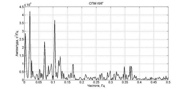
It describes the periodogram method of using FFT. In addition, there is the Welch method, autoregression, etc.
Based on the data obtained, the PSD calculates the powers of the HF, LF, VLF signal components, as well as the total power TP. In accordance with the recommendations, the ranges will be limited to the following frequencies.
To calculate the power component is used trapz function. The function I = trapz (y) calculates the integral, assuming that the integration step is constant and equal to one; in the case when the step h is different from one but is constant, a sufficiently calculated integral multiplied by h. In this case, h = (fInt / N), where fInt = 4 Hz is the sampling frequency, N is the number of calculated FFT bins.
The data obtained is sufficient for calculating the frequency parameters of PARS using known formulas.
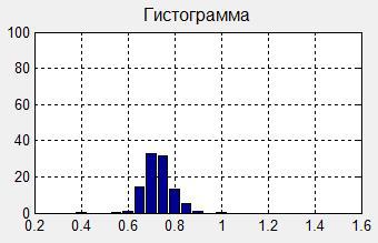
We define the geometric parameters of the histogram. For this, in accordance with the recommendations, the banding ranges of cardiointervals are indicated and the hist command is used.
The result of the construction is shown in the figure.
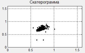
Build a scattergram.
PS: Since I am not a medical specialist, in terms I admit possible inaccuracies.
The described principle of the analysis appeared on the basis of the sources I found and the developments that have already been made publicly available.
Due to the peculiarities of the genre, the material attempted to concisely concisely, omitting some technical points of MATLAB.
I will be glad to constructive criticism and try to answer possible questions. I hope the material will be useful to someone. Thanks for attention!
Quite accessible and basic about research methods
Baevsky R.M. and others. Analysis of heart rate variability using different electrocardiographic systems
Measurement standards and recommendations for the analysis of HRV
The database of records RR-intervals from PhysioNet
Ready-to-use MATLAB features: Software for Heart Rate Variability
HRV analysis is based on the determination of the sequence of RR intervals of ECG, i.e. between two consecutive heartbeats. They also use the concept of NN-intervals (normal-to-normal), that is, here only the intervals between normal contractions are taken into account (the analysis does not include the intervals recorded during heartbeat disturbances, as well as those resulting from external interference).
The upper graph of the figure illustrates the process of detecting the duration of RR-intervals on the ECG.
The patient after the examination receives a cardiointervalogram (CIG), which is a set of RR-intervals (the lower graph of the figure, which are displayed one after the other. Here the pulse height is equal to the duration of the corresponding RR interval in ms, and the time of appearance of the next pulse corresponds to the time of its detection.
')
Currently, there are several methods for assessing HRV. Among them are three groups:
- time-domain methods - based on statistical methods and directed to the study of general variability;
- autocorrelation analysis and correlation rhythmography - integral indices of HRV;
- frequency domain methods - the study of the periodic components of HRV.
In this regard, various methods of analysis of HRV use different qualitative and quantitative assessment criteria. Sometimes there is a contradiction in the interpretation of data obtained on the basis of various methods for assessing heart rate. Therefore, the current methods are the total assessment of indicators of HRV. R. M. Baevsky proposed for an integrated assessment of the heart rhythm an indicator of the activity of regulatory systems (PARS), which is calculated in points based on the listed techniques. Those. Qualitative analysis of HRV should be carried out using all three methods, and the data obtained are used to calculate the PARS index.
The initial data for the analysis is the recording of successive instants of time for the appearance of the next R-wave. For the analysis, more often 5-minute records are used, although there are options for analyzing records of a different length.
To build CIG, it is necessary to know not only the moments of appearance of the R-wave on the ECG, but also the length of time between two adjacent R-teeth. To calculate this duration, use the MATALAB diff function, which calculates the finite differences.
RR = diff(D_times); % RR-. D_times – R-, times = D_times(2:(length(D_times))); % . Further, it is necessary to determine the possible RR-intervals that are not normal (get NN-intervals). To do this, we first form a unit vector of flag values for each RR interval:
flags = ones(max(size(RR)),1); % RR-. Now the elements of the flags (flags) vector that correspond to the “abnormal” RR-intervals are replaced by zeros. Moreover, anomalous intervals will have to be detected manually.
To do this, we construct the CIG of the signal under study using the stem function.
stem (RR, 'Marker','.', 'color', [0 0 0]), title (' ', 'FontSize', 12); xlabel(' ','FontSize',12); ylabel(', .','FontSize',12); The figure shows a fragment of a construction with an anomalous (non-sinus rhythm) interval, which cannot be taken into account in further calculations.
Such intervals are removed from the CIG, and the areas of their removal will be interpolated by the linear method according to the value of the neighboring intervals. This approach allows you to create a sequence of NN without disturbing the overall dynamics of the signal. However, it should be noted that the result of the CIG analysis will be satisfactory with a false interval of not more than 5-6.
To recover deleted intervals, we use the MATLAB function for one-dimensional table interpolation. Syntax:
RRinterp = interp1 (x, y, xi, '<method>').
In this case, we assume x is the time of occurrence of neighboring false (or a group of false) intervals, y is their duration, xi is the time of appearance of false intervals marked flags, '<method>' - 'linear'. As a result, the variable RRinterp returns the duration of the interpolated intervals.
In the next step, it is necessary to obtain from uneven CIG fig. 3 uniformly sampled signal using the smooth interpolation method. For this it is recommended to use interpolation by cubic splines. The recommended sample rate for uniform sampling is 4 Hz.
fInt = 4; % / xSpline = min(times): 1/fInt: max(times); % / RRspline = interp1(times, RRint, xSpline, 'spline'); % . times – , RRint – NN-. To conduct a frequency analysis of the processed CIG RRspline signal, it is necessary to get rid of its constant component, i.e. remove linear trend. This is achieved by subtracting from the samples of the RRspline signal its arithmetic average value.
RRdetrend = RRspline - mean (RRspline);
The result is shown in the figure.
To carry out frequency analysis (calculation of the spectral power density), it is necessary to perform the procedure of the discrete Fourier transform (DFT). At the same time, it is necessary to minimize spectrum leakage and scalloped distortion. For this, we apply the window weighting method. It is recommended to use the Tukey window with 25% anti-aliasing.
w = tukeywin(length(rrdetrend), 0.25); % 25% . rrdetrend = (w'.*rrdetrend).*1000; % . And also we implement the addition with zeros.
Pspectr = fft(rrdetrend, 2048); % 2^11. The result of the calculation of the PSD of the analyzed CIG signal, calculated on the basis of the FFT algorithm, is shown in the figure.
It describes the periodogram method of using FFT. In addition, there is the Welch method, autoregression, etc.
Based on the data obtained, the PSD calculates the powers of the HF, LF, VLF signal components, as well as the total power TP. In accordance with the recommendations, the ranges will be limited to the following frequencies.
BW = [0.003 0.04; ... % , VLF 0.04 0.15; ... % , LF 0.15 0.4]; % , HF To calculate the power component is used trapz function. The function I = trapz (y) calculates the integral, assuming that the integration step is constant and equal to one; in the case when the step h is different from one but is constant, a sufficiently calculated integral multiplied by h. In this case, h = (fInt / N), where fInt = 4 Hz is the sampling frequency, N is the number of calculated FFT bins.
The data obtained is sufficient for calculating the frequency parameters of PARS using known formulas.
We define the geometric parameters of the histogram. For this, in accordance with the recommendations, the banding ranges of cardiointervals are indicated and the hist command is used.
dRR = 0.4: 0.05: 1.3; % [ampRR, dRR] = hist (RRspline, dRR); % ampRR_proc = (ampRR.*100)./length(rrspline); % [yMo, yi] = max (ampRR); Mo = dRR(yi); % - AMo = (yMo*100)/length(RRspline); % MxDMn = (max(RRspline) - min(RRspline)); % bar (dRR, ampRR_proc), grid on % . title ('', 'FontSize', 12); ylabel('%','FontSize',12); axis ([0.2 1.6 0 100]) The result of the construction is shown in the figure.
Build a scattergram.
rr1 = RRspline (1 : 2:end); % () RR(n) rr2 = RRspline (2 : 2: end); % () RR(n+1) if length(rr1) ~= length(rr2) if length(rr1) > length(rr2) rr1 = rr1 (1: end - 1); else rr2 = rr2 (1: end - 1); end end plot (rr1, rr2,'Marker','.','LineStyle','none','Color',[0 0 0]) title ('', 'FontSize', 12), grid on axis ([0 1.6 0 1.6]) PS: Since I am not a medical specialist, in terms I admit possible inaccuracies.
The described principle of the analysis appeared on the basis of the sources I found and the developments that have already been made publicly available.
Due to the peculiarities of the genre, the material attempted to concisely concisely, omitting some technical points of MATLAB.
I will be glad to constructive criticism and try to answer possible questions. I hope the material will be useful to someone. Thanks for attention!
Sources
Quite accessible and basic about research methods
Baevsky R.M. and others. Analysis of heart rate variability using different electrocardiographic systems
Measurement standards and recommendations for the analysis of HRV
The database of records RR-intervals from PhysioNet
Ready-to-use MATLAB features: Software for Heart Rate Variability
Source: https://habr.com/ru/post/257345/
All Articles