RS analysis (analysis of the fractal structure of time series)
Standard Gaussian statistics work based on the following assumptions. The central limit theorem states that as the number of tests increases, the limit distribution of a random system will be a normal distribution. Events should be independent and identically distributed (i.e. they should not affect each other and should have the same probability of occurrence). In the study of large complex systems, a hypothesis about the normality of the system is usually assumed, so that standard statistical analysis can be applied further.
Often in practice, the systems studied (from sunspots, average annual precipitation to financial markets, time series of economic indicators) are not normally distributed or close to it. For the analysis of such systems, Hurst [1] proposed the method of Normalized scope (RS-analysis). Mainly this method allows us to distinguish between random and fractal time series, as well as to draw conclusions about the presence of non-periodic cycles, long-term memory, etc.
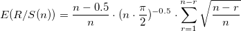
Next, we check the obtained result for significance. To do this, we check the hypothesis that the analyzed structure is normally distributed. R / S are random variables, normally distributed, then it can be assumed that H are also normally distributed. The asymptotic limit for an independent process is the Hurst index of 0.5. Enis and Lloyd [2], as well as Peters [3], suggested using the following expected R / S ratios:
For n observations, we find the expected Hurst index: .
.
The expected variance will be as follows: where T is the number of observations in the sample.
Custom statistics: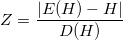 .
.
We compare it with the critical value of the normalized normal distribution.
If the sample value is less than the critical value, then the hypothesis about the normal distribution of the system is not rejected at this level of significance. The structure is random and has a normal distribution law.
Often in practice, the systems studied (from sunspots, average annual precipitation to financial markets, time series of economic indicators) are not normally distributed or close to it. For the analysis of such systems, Hurst [1] proposed the method of Normalized scope (RS-analysis). Mainly this method allows us to distinguish between random and fractal time series, as well as to draw conclusions about the presence of non-periodic cycles, long-term memory, etc.
RS analysis algorithm
- Given the original series
 . Calculate logarithmic relations:
')
- Split a row
 on
on  adjacent periods of length
  . Mark each period as
  where
where  . We define for each average value:
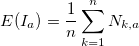
- Calculate the deviations from the average for each period :
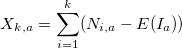
- Calculate the scale within each period:

- Calculate the standard deviations for each period. :

- Each
 divide by
  . Next, we calculate the average value of R / S :
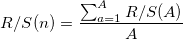
- Increase and repeat steps 2-6 until

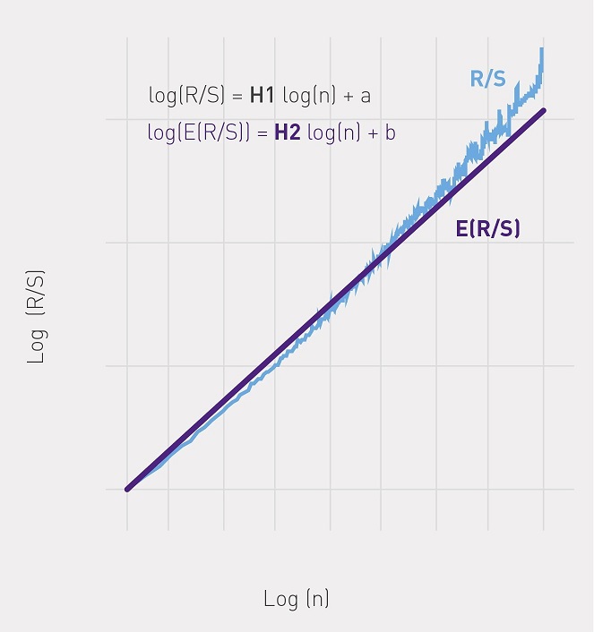
- Build a dependency graph
 from
from  and using the OLS find the regression of the form:
  where H is the Hurst index (see figure).
Significance test
Next, we check the obtained result for significance. To do this, we check the hypothesis that the analyzed structure is normally distributed. R / S are random variables, normally distributed, then it can be assumed that H are also normally distributed. The asymptotic limit for an independent process is the Hurst index of 0.5. Enis and Lloyd [2], as well as Peters [3], suggested using the following expected R / S ratios:
For n observations, we find the expected Hurst index:
.The expected variance will be as follows:
where T is the number of observations in the sample.Custom statistics:
.We compare it with the critical value of the normalized normal distribution.
If the sample value is less than the critical value, then the hypothesis about the normal distribution of the system is not rejected at this level of significance. The structure is random and has a normal distribution law.
Bibliography:
- Hurst, G.E., 1951. “Long-term reservoir capacity”. Proceedings of the American Society of Civil Engineers, 116, 770-808.
- Anis, AA, Lloyd, EH (1976) Hurst range of independent normal summands. Biometrica 63: 283-298.
- Peters, EE (1994) Fractal Market Analysis. Wiley, New York. ISBN 0-471-58524-6.
Source: https://habr.com/ru/post/256381/
All Articles