Machine Learning - 4: Moving Average
It is considered that the two basic operations of “machine learning” are regression and classification. Regression is not only a tool for identifying the y (x) dependency parameters between the x and y data series (to which I have already devoted several articles ), but also a special case of the smoothing technique. In this example, we will go a little further and consider how smoothing can be carried out when the type of the dependence y (x) is not known in advance, as well as how to filter the data that are controlled by different effects with significantly different temporal characteristics.
One of the most popular smoothing algorithms used, in particular, in stock trading, is sliding averaging (I include it in a series of articles on machine learning with some stretch). Consider moving averaging using the example of dollar fluctuations over the past few weeks (again, using Mathcad as a research tool). The calculations themselves are here .
')
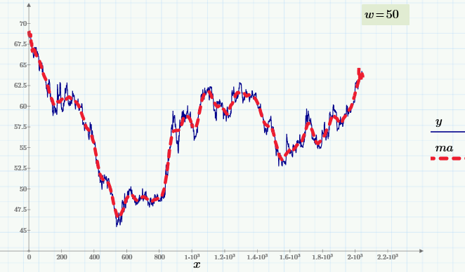
The above chart shows the exchange value of the dollar against the ruble with an interval of 1 hour. The original data is represented by a blue curve, and the smoothed data is red. Even with the naked eye it can be seen that rate fluctuations have several characteristic frequencies, which is the subject of one of the directions of technical analysis of markets.
Smoothing with “moving average”
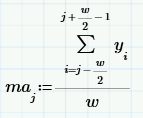
The smoothing principle based on the "moving average" (MA - from the English. "Moving average") is to calculate for each value of the argument y i the average value of the neighboring w data.
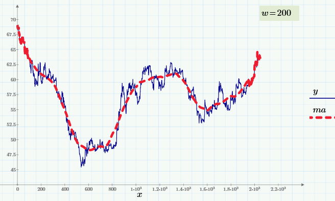
The number w is called the sliding averaging window : the larger it is, the more data are involved in calculating the average, respectively, the smoother the curve is. In the upper figure, the window is w = 50, but this is how sliding averaging will look like when w = 200.
How does the Fourier spectrum of data change with averaging?
Obviously, for small w, the smoothed curves practically repeat the course of data changes, and for large w, they reflect only the regularity of their slow variations. This is a typical example of data filtering, i.e. eliminate one of the components of the dependence y (x i ). The most common goal of filtering is to suppress fast variations of y (x i ), which are usually caused by noise. As a result, another rapidly smoothed dependence is obtained from the rapidly oscillating dependence y (x i ), in which the lower-frequency component dominates.
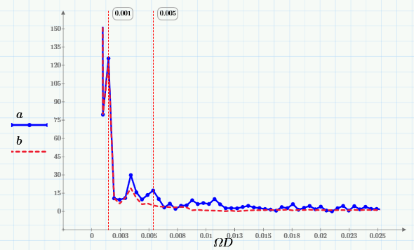
These arguments smoothly translated us to the terminology of the spectra. Let's draw a graph of the Fourier transform ( "Fourier spectrum" ) of the source data:
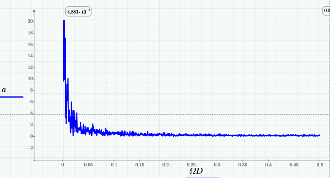
and make sure that the moving average spectrum cuts out high frequencies from it (starting at about 0.005 Hz):
Explanation: Fourier spectrum of the sum of sines and its MA
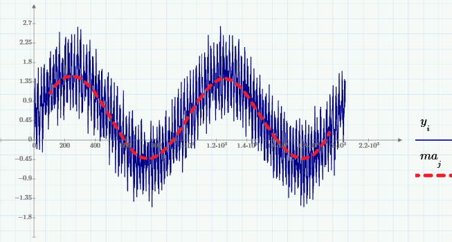
In order to clarify the principle of calculating the Fourier spectrum, instead of (random) input data, we consider a simple model of the sum of several deterministic signals (sinusoids with different frequencies and amplitudes) and pseudo-random noise:

Here are the graphs of this sum and its MA (with the same window w = 200):
and their Fourier spectra:
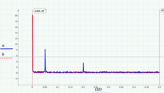
It can be seen from them that moving averaging cuts out high frequencies from the signal, starting with a frequency of 0.005 Hz. This is best seen in the close-up of the low-frequency region of the spectrum:

Thus, choosing a suitable window, you can shift the region of suppressed frequencies in the right direction (the more w, the farther this boundary shifts to the left).
Bandpass filtering
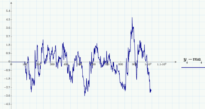
Let us return to stock analytics and demonstrate an extremely simple way of cutting out the necessary frequency band from the source data. Namely, in contrast to suppressing noise (the high-frequency component), the opposite problem is often considered - the elimination of slowly varying variations (sometimes this problem is called trend elimination , or detrending ). Using sliding averaging, it is very simple to implement it — by subtracting from the MA signal (with a selected window):
Also of interest are the mixed tasks of isolating medium-scale variations by suppressing both faster and slower variations. One of the solution possibilities is associated with the use of “bandpass filtering” , which is implemented as follows:
1. Elimination of the high-frequency component from the signal y, aimed at obtaining a smoothed signal from the middle, for example, using sliding averaging with a small window (for example, w = 200).
2. The selection from the signal of the middle low-frequency component of the slow, for example, by sliding averaging with a large window w.
3. Subtracting from the signal the middle trend is slow, thereby highlighting the medium-scale component of the original signal y.
I leave to the interested reader the opportunity to implement bandpass filtering in Mathcad Express myself (with a slight reservation that in the free version of Matkad, the FFT algorithm for calculating Fourier spectra is disabled and it will not work). The calculations themselves are here .
Literature:
1. Kiryanov D.V., Kiryanova E.N. Computational Physics ( PDF , ch. 1, p. 6 and 7). M .: Polybuk Multimedia, 2006.
2. Bath M. Spectral analysis in geophysics. M., Science, 1980.
One of the most popular smoothing algorithms used, in particular, in stock trading, is sliding averaging (I include it in a series of articles on machine learning with some stretch). Consider moving averaging using the example of dollar fluctuations over the past few weeks (again, using Mathcad as a research tool). The calculations themselves are here .
')
The above chart shows the exchange value of the dollar against the ruble with an interval of 1 hour. The original data is represented by a blue curve, and the smoothed data is red. Even with the naked eye it can be seen that rate fluctuations have several characteristic frequencies, which is the subject of one of the directions of technical analysis of markets.
Smoothing with “moving average”
The smoothing principle based on the "moving average" (MA - from the English. "Moving average") is to calculate for each value of the argument y i the average value of the neighboring w data.
The number w is called the sliding averaging window : the larger it is, the more data are involved in calculating the average, respectively, the smoother the curve is. In the upper figure, the window is w = 50, but this is how sliding averaging will look like when w = 200.
How does the Fourier spectrum of data change with averaging?
Obviously, for small w, the smoothed curves practically repeat the course of data changes, and for large w, they reflect only the regularity of their slow variations. This is a typical example of data filtering, i.e. eliminate one of the components of the dependence y (x i ). The most common goal of filtering is to suppress fast variations of y (x i ), which are usually caused by noise. As a result, another rapidly smoothed dependence is obtained from the rapidly oscillating dependence y (x i ), in which the lower-frequency component dominates.
These arguments smoothly translated us to the terminology of the spectra. Let's draw a graph of the Fourier transform ( "Fourier spectrum" ) of the source data:
and make sure that the moving average spectrum cuts out high frequencies from it (starting at about 0.005 Hz):
Explanation: Fourier spectrum of the sum of sines and its MA
In order to clarify the principle of calculating the Fourier spectrum, instead of (random) input data, we consider a simple model of the sum of several deterministic signals (sinusoids with different frequencies and amplitudes) and pseudo-random noise:
Here are the graphs of this sum and its MA (with the same window w = 200):
and their Fourier spectra:
It can be seen from them that moving averaging cuts out high frequencies from the signal, starting with a frequency of 0.005 Hz. This is best seen in the close-up of the low-frequency region of the spectrum:
Thus, choosing a suitable window, you can shift the region of suppressed frequencies in the right direction (the more w, the farther this boundary shifts to the left).
Bandpass filtering
Let us return to stock analytics and demonstrate an extremely simple way of cutting out the necessary frequency band from the source data. Namely, in contrast to suppressing noise (the high-frequency component), the opposite problem is often considered - the elimination of slowly varying variations (sometimes this problem is called trend elimination , or detrending ). Using sliding averaging, it is very simple to implement it — by subtracting from the MA signal (with a selected window):
Also of interest are the mixed tasks of isolating medium-scale variations by suppressing both faster and slower variations. One of the solution possibilities is associated with the use of “bandpass filtering” , which is implemented as follows:
1. Elimination of the high-frequency component from the signal y, aimed at obtaining a smoothed signal from the middle, for example, using sliding averaging with a small window (for example, w = 200).
2. The selection from the signal of the middle low-frequency component of the slow, for example, by sliding averaging with a large window w.
3. Subtracting from the signal the middle trend is slow, thereby highlighting the medium-scale component of the original signal y.
I leave to the interested reader the opportunity to implement bandpass filtering in Mathcad Express myself (with a slight reservation that in the free version of Matkad, the FFT algorithm for calculating Fourier spectra is disabled and it will not work). The calculations themselves are here .
Literature:
1. Kiryanov D.V., Kiryanova E.N. Computational Physics ( PDF , ch. 1, p. 6 and 7). M .: Polybuk Multimedia, 2006.
2. Bath M. Spectral analysis in geophysics. M., Science, 1980.
Source: https://habr.com/ru/post/256317/
All Articles