Introduction

Computer math systems (SKA) work wonders. The development of mathematical packages has reached the level when the thought involuntarily creeps in - why do we need classical methods of teaching mathematics (or physics, or mechanics) at school or university, if most of the dirty work on transforming expressions can be passed on to the machine’s shoulders. And if it is impossible, or it is difficult to get an analytical solution of the problem, then why not “click it out” numerically in one of the popular packages. So, let's limit the level of students' understanding to the compilation of the initial system of equations, and we will not solve it, everything will be easily and easily done by a computer for them.

I will not hide the fact that the catalyst for writing this post was an article about the problem of two old women, walkers, taken from the book by V.I. Arnold. In this regard, the idea appeared to consider a simple mathematical problem, the solution of which shows that the capabilities of the SKA often rest on a fairly natural upper limit, and to obtain a compact solution suitable for further analysis, it is necessary to straighten the convolutions slightly.

1. The system of trigonometric equations

When, in the not too distant 2003, I began working on my PhD thesis, I was faced with the need to solve a system of trigonometric equations of the form


')


The parameters a, b, A, B are positive. Conditions are imposed on the roots of the equation



Where do we encounter such systems? When calculating the kinematics of closed four-links, for example. Such a closed four-chin was in my work, almost the same as I got about a year ago, when I undertook to make a “sabbath” (helped one professor in his work).

Then, in 2003, I only became acquainted with the Maple system and was delighted with its capabilities; naturally, I assigned this system to it. And I was waiting for a "bummer" ... Let's see what solution Maple 18 and Mathematica 10 give for this task today.

2. Solution of the problem in the SKA "head on"

In my favorite Maple we set the system of equations

restart; eq01 := a*cos(x) + b*cos(y) = A; eq02 := a*sin(x) - b*sin(y) = B; 

and try to solve

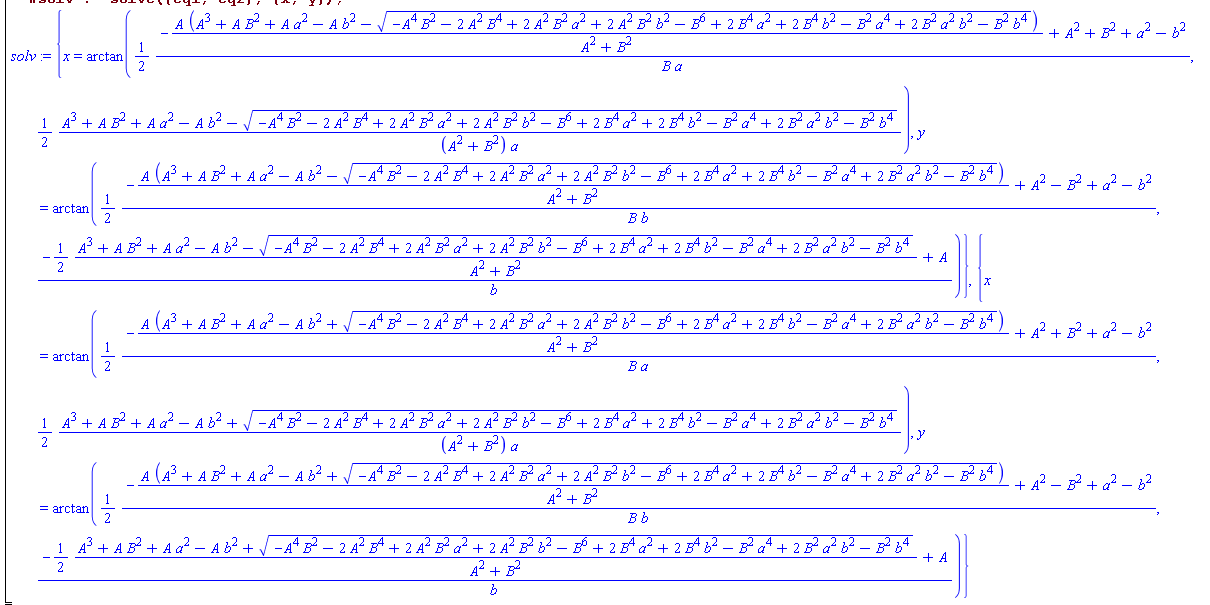
 solv := solve({eq01, eq02}, {x, y}); 

and we get ...

This bjaka did not fit into the online LaTeX, so I had to bring a screenshot. This result is obtained because the problem statement is too general. It is necessary to indicate to the system which solution interests us using the condition (3)

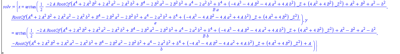
 solv := solve({eq1, eq2, x > 0 and x < Pi, y > 0 and y < Pi}, {x, y}); 

In this case, the result looks better.



Once again I will apologize to the reader for the clumsy screenshot and note that we have received two solutions of the system (1) - (3) and we now have yet to figure out what answer corresponds to the mechanical meaning of the problem (it is there, yes), and considering that for a, b, A, and B can be quite significant expressions (not depending, of course, on x and y), we should be pretty sad at this moment.

Mathematica 10 with these equations has a better situation in the sense that it gets the final form of a general solution, part of which is on the screen


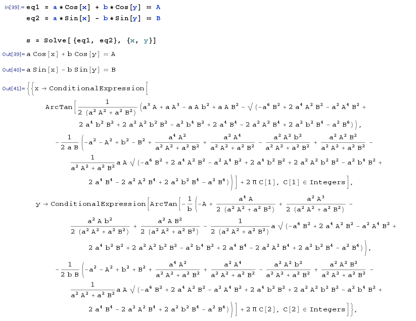
If the system is supplemented with the condition (3), then Wolfram tells us that Solve [...] does not have a solution method for such a case (I would be grateful to the reader for a hint on this issue, because I consider that I myself did not study the question completely, but for now I will continue the story).

In addition, both SKA issue in the decision godless arctangent, which is not always convenient for different reasons, which I will not talk about - in each case, their reasons.

When my late “chief” saw these decisions in 2003, he thought and said that “these crocodiles should be combed”, which made me plunge into further thought. And I again armed myself with a piece of paper and a pencil ...

3. SKA + brain

To obtain a fairly compact solution, it is necessary to transform the system (1) - (3) to a linear one with respect to unknowns. To do this, use the school knowledge of trigonometry.

So, we will raise equations (1) and (2) into a square and add, transferring everything that does not depend on x and y to the right side of the equation

 left1 := lhs(eq01): left2 := lhs(eq02): right1 := rhs(eq01): right2 := rhs(eq02): eq03 := simplify(left1^2 + left2^2)= right1^2 + right2^2; eq03 := eq03 - (a^2 + b^2); left3 := combine(lhs(eq03)); eq03_1 := left3 = rhs(eq03); 

using the formula "cosine of the sum", we get a new equation



Now, solving it with respect to the sum of the unknowns, we arrive at a linear equation



Linear equation is linear in Africa as well. Finding one unknown, we get another. Let us deal with another unknown, eliminating x from one of their equations. Since we have condition (3), it is obvious that



and this gives us the opportunity to use the basic trigonometric identity without the plus or minus ambiguity



Cosine X take from the first equation



thus obtaining for sine X



In order not to puff paper, we will entrust all this to Maple.

 eq01_1 := subs(cos(x) = u, eq01); slv := solve(eq01_1, u); eq02_1 := subs(sin(x) = sqrt(1-slv^2), eq02); eq02_1 := eq02_1 + b*sin(y); 

having an equation



Equation (7) should be squared and some transformations should be made.

 left := expand(lhs(eq02_1)^2): right := expand(rhs(eq02_1)^2): eq02_2 := collect(simplify(right - left), b); eq02_3 := subs(coeff(eq02_2, b) = tmp, eq02_2); slv2 := solve(eq02_3, tmp); eq02_4 := -2*A*cos(y) + 2*B*sin(y) = slv2; eq02_5 := eq02_4/(-2); 

coming to the form equation


And now we will execute, known to many, "feint ears"

 left2 := lhs(eq02_5); left3 := subs(A = O2A*cos(xi), B = O2A*sin(xi), left2); left4 := subs(O2A = sqrt(A^2 + B^2), combine(left3)); 

that is, we divide both sides of the equation by and collapse the left-hand side using the cosine sum formula, rightly assuming that



We get a new equation,



which successfully decide on y

 eq02_6 := left4 = rhs(eq02_5); slv3 := subs(xi = arccos(A/sqrt(A^2 + B^2)), solve(eq02_6, y)): 

As you can see, the game came out quite compact. We return to equation (5) and find x



And now comparing the obtained with the above "crocodiles", we will do

findings

Computer algebra systems are an indispensable assistant of a modern scientist, simplifying his life and eliminating the need to burrow into the “sheets” of solutions on paper, relieving from annoying errors / errors, freeing the brain for productive activities. But, their successful application is inseparable from the general mathematical culture and knowledge of elementary things. Otherwise, the solution lying on the surface has a chance to never see the light.

Thank you for your attention to my writing!