Signal detection in noise

By the nature of my business, I have to monitor various parameters of ground-based pulse-phase radio navigation systems (IFRNS) Chaika and Loran-C. In this article I want to share one of the methods for detecting the arrival time of an IFRNS pulse in the presence of noise. The method is applicable to many problems of searching for a signal of a known form.

The systems belong to the class of hyperbolic systems and are based on measuring the difference in arrival time of radio pulses received from a chain of transmitting stations. In each chain, one of the stations is leading, and the others are driven. All of them are synchronized exactly .

The main problem in detecting signals of the IFRS is the distortion of the shape of the received radio pulses due to the superposition of the reflected components on the surface wave. Signal components that do not propagate along the surface go through different paths at different times. It is impossible to reliably predict the time of their arrival. However, it is obvious that the reflected signal components propagate more slowly than the surface component. They also affect the shape of the received signal. The form of the received radio pulse may vary depending on the season, time of day, as well as weather conditions and geographic location. To perform the tasks of navigation, an algorithm is needed to select the beginning of the surface component of the radio pulse.

The received signal x _t (t) in the time domain can be represented by the following equation:
(one)
')
where x _g (t) is the surface component, the amplitude and delay of the nth reflected component are determined by the coefficients k _n and t _n , and e (t) is the noise component.
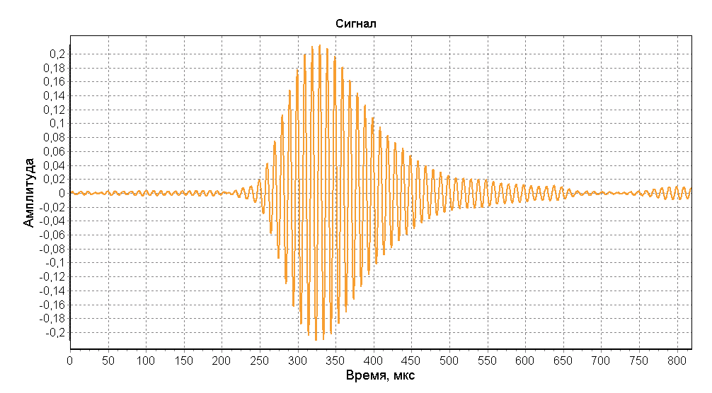
Below shows the reference pulse IFRS and its spectrum after passing through the receiver bandpass filter. The sampling rate is 5 MHz.




As an example, consider a simulated radio pulse consisting of surface and reflected components. The pictures below are graphs showing a pulse model consisting of two components displaced from each other by 130 µs. The amplitude of the reflected component is 2 times lower than the amplitude of the surface component.




The equivalent signal representation in the frequency domain is described as:
(2)

where X _t (f) , X _g (F) and E (f) are the spectra of the signals x _t (t) , x _g (t) and e (t) .
We assume that the spectrum of the reference normalized signal of the system "Loran-S" or "Seagull" is denoted as X ₀ (f) .
It's obvious that
(3)

where k _g is the amplitude of the surface component. If the expression for X _g (f) from formula (3) is substituted into formula (2) and divided by term all the terms on X ₀ (f) , we get the expression
(four)

The figure below shows a graph of the result of dividing the spectrum of the signal by the spectrum of the standard. Pictured in red, the graph is a horizontal sawtooth line in the entire frequency range.


The inverse Fourier transform over the expression (4) gives the formula
(five)

The mathematical meaning of expression (5) is that in the time domain we get the peaks in the form of delta functions at the moments when both the surface and all reflected signal components appear, normalized in amplitude.
The figure below shows the graph of detection of the beginning of the signal components. As can be seen from the graph, the ratio of the amplitudes of the signal components is two and the distance between the peaks is 130 μs, which corresponds to the parameters of the constructed model.



The conventional spectral division method works well for ideal signals. When a noise component is added to a signal, the efficiency of the method deteriorates dramatically. The figures below show the graph of detection of the beginning of the signal at a signal-to-noise ratio of 25 dB. As can be seen from the figures, the definition of the beginning of the signals cannot be performed.



On the spectrum graph, it can be seen that within a band of approximately 30 kHz with a center at a point of 100 kHz, the result of dividing the spectra has a horizontal sawtooth shape as when using the method of dividing spectra on an ideal, non-noisy signal. Using a 30 kHz rectangular window with a center at 100 kHz eliminates the effects of noise before the inverse Fourier transform operation. The figure below shows a graph of detection of the beginning of a signal when using window filtering of a noisy signal. Two maximums of the graph allow to detect the beginning of each of the signal components against the background of noise and also to estimate the ratio of their amplitudes.


The method of dividing spectra using window smoothing is effective when the signal-to-noise ratio is above 12 dB. The most effective type of window is recognized as a rectangular window with a band of 30 kHz. The pictures below show the real momentum of the Northern Sea of ​​China Chain and the schedule for detecting its onset.




The original article is located here . The algorithm is currently used by me to monitor the parameters of the stations of the IFRS of the Far Eastern region.