Best approaches to moving a MATLAB code to a fixed point
When converting a project from a floating point to a fixed point, engineers must determine the optimal data types at a fixed point. These data types must meet the constraints of embedded hardware, while meeting the system requirements for computational accuracy. Fixed-Point Designer helps you develop algorithms at a fixed point and convert algorithms from floating point to fixed point, automatically suggesting data types and arithmetic attributes at a fixed point. At the same time, it is possible to compare simulation results at a fixed point up to a bit with the reference results at a floating point.
This article outlines best practices for preparing a MATLAB code for conversion, directly converting a MATLAB code to a fixed point, and optimizing algorithms for efficiency and performance. If you develop algorithms at a fixed point in MATLAB for later manual code writing or convert to a fixed point for automatic code generation, then the described techniques will help you turn your general-purpose MATLAB code into efficient code at a fixed point.
Preparing the code for transfer to a fixed point
There are three steps to take to ensure a smooth conversion process:
')
Separation of the main algorithm from the rest of the MATLAB code
Usually the algorithm is accompanied by a code that prepares the input data and a code that creates graphs for verifying the results. Since only the core of the algorithm needs to be converted to a fixed point, it will be more efficient to structure the code so that a separate test file creates inputs, calls the main algorithm and draws graphs of the results. In this case, the main algorithm will also be in a separate file or files (Table 1).
Table 1. Code before and after the separation of the main algorithm from the test strapping.
Preparation of algorithmic code for instrumentation and acceleration
Instrumentation and acceleration simplify the conversion process. Fixed-Point Designer is used to instrument code and record the minimum and maximum values of all named and intermediate variables. This tool can use recorded values to suggest data types for use in fixed point code.
Using Fixed-Point Designer, you can also speed up algorithms at a fixed point by creating a MEX file, and speed up the simulations required to verify the implementation at a fixed point relative to the original version.
Instrumentation and acceleration rely on code generation technology, so before using them, you need to prepare the algorithm for generating code - even if you do not plan to use MATLAB Coder or HDL Coder to generate C code or HDL code.
First, you need to define functions or constructions in your MATLAB code that are not supported for generating code (see Language Support for a list of supported functions and objects).
There are two ways to automate this step:
After preparing the algorithm for generating code, you can use the Fixed-Point Designer to instruct and speed up the code. Use
Checking the support of a fixed point functions used in the algorithmic code
If you identify a function that is not supported for generating code, you have three options:
Then you can continue converting the code to a fixed point, and return to the unsupported function when you have a suitable replacement (Table 2).
Table 2. Code before and after isolation of an operation in a floating point using a type conversion (reverse type conversion to a fixed point at the output is not shown).
Managing data types and limiting the growth of bit depth
In a fixed-point implementation, variables at a fixed point must remain in arithmetic with a limited width and must not arbitrarily turn into a floating point. It is also important to prevent the growth of digit capacity .
For example, consider the following code:
This expression overwrites y with the value
Use the syntax to preserve the data type y.
Table 3. Code before and after using index assignment to prevent the growth of digit capacity.
Creating a table with types to separate data type definitions and algorithmic code
Separating data type definitions and algorithmic code simplifies the comparison of implementations at a fixed point and the transfer of the algorithm to other target equipment.
To apply this best practice, do the following:
Table 4a. The code before and after creating the data type table to separate the algorithmic code from the type definitions.
Table 4b. Code before and after adding a single precision data type to the type table.
Adding data types at a fixed point in the type table
After creating a table with data type definitions, you can add data types at a fixed point based on your conversion goals to a fixed point. For example, if you plan to implement an algorithm in C, the word size of data types at a fixed point will be limited to multiples of 16. On the other hand, if you plan to implement in HDL, the word size is not limited.
To get a set of suggested data types for your code, use the commands Fixed-Point Designer.

Figure 1. The code generation report created by showInstrumentationResults with the proposed data types for variables in the filtering algorithm.
Then you can customize the proposed types if necessary (Tables 5 and 6).
Table 5. A filtering algorithm and a test script for instrumenting and executing code and displaying the proposed data types at a fixed point for variables.
Table 6. Test script and filtering algorithm from Table 4 with data types at a fixed point.
Run your algorithm with new data types at a fixed point and compare the output with the results of the reference algorithm at the floating point.
Data type optimization
Whether you chose your own types at a fixed point or used the proposed Fixed-Point Designer, always look for opportunities to optimize word sizes, fractional sizes, signality, and perhaps even fimath modes. This can be done using scaled doubles by examining a histogram of variable values or by testing various types of data from your type table.
Use scaled doubles to identify potential overflows
Scaled doubles are hybrids of numbers in a floating point and a fixed point. Fixed-Point Designer stores scaled doubles in the form of double precision numbers, but retains information about the word width, sign and word length. To use scaled doubles, you need to set the data type overwriting property (DTO) (Table 7).
Table 7. Methods for setting the data type rewriting property locally and globally.
Remember to reset the global DTO if it is no longer needed with the command
Use buildInstrumentedMex to run your code and showInstrumentationResults to view the results. In the code generation report, the values that would overflow are highlighted in red (Figure 2).
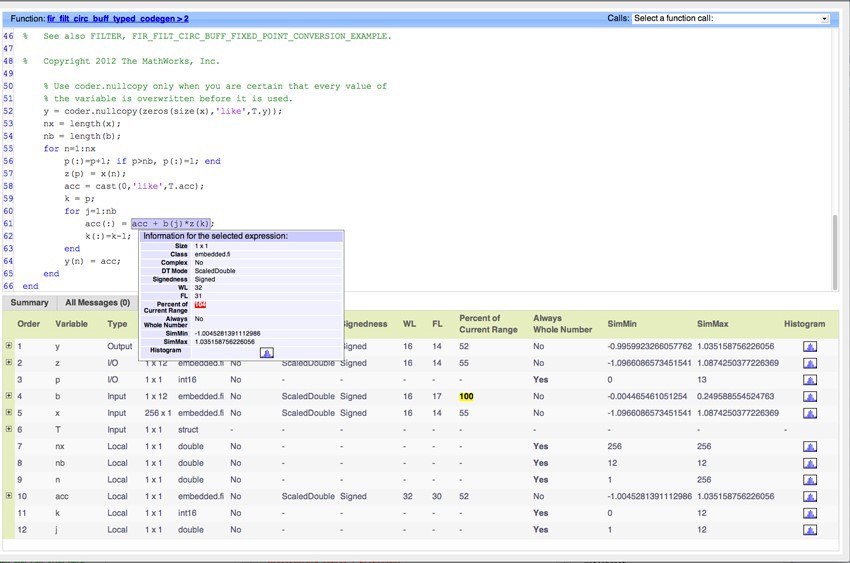
Figure 2. Code generation report showing overflows using Scaled Doubles type (left) and histogram icon (right).
Checking the distribution of variable values
You can use the histogram to identify data types with values that are within the allowable range, out of range or below resolution (accuracy). By clicking on the histogram icon, you can run the NumericTypeScope and see the distribution of the values observed during the simulation for the selected variable (Figure 3).
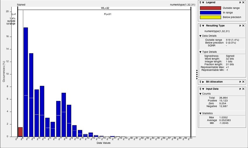
Figure 3. A histogram showing the distribution of values of a variable that overflows (“Outside range”), shown in red.
Testing various data types from a type table
You can add your own variations of data types at a fixed point in the type table (Table 8).
Table 8. Test script to study the effects of using different types of data at a fixed point from the type table for the filtering function.
Comparison of the results of different iterations to verify the accuracy of the algorithm after each change (Figure 4).

Figure 4. Graphs of the test script results from Table 8, showing the output and error after converting to 8-bit and 16-bit data types at a fixed point.
Algorithm optimization
There are three most common ways to optimize your algorithm to improve performance and generate more efficient C code.
You can:
Using fimath properties to improve the efficiency of generated code
When using the fimath default settings, additional code can be generated to implement saturation during overflow, rounding, and arithmetic with complete precision (Table 9a).
Table 9a. The original MATLAB code and C code generated with fimath default settings.
To make the generated code more efficient, you need to select such fixed-point arithmetic settings that are appropriate for your processor types. Use the fimath properties to describe arithmetic, rounding methods, and overflow actions to define rules for performing arithmetic operations on your fi objects (Table 9b).
Table 9b. The original MATLAB code and C code generated with fimath settings appropriate to the processor types.
Replacing built-in functions with fixed point implementations
Some MATLAB functions can be replaced to achieve a more efficient implementation at a fixed point. For example, you can replace the built-in function with an interpolation table or a CORDIC implementation, which only requires iterative shift and sum operations.
The implementation of division operations in other ways
Division operations are often not fully supported by the hardware, and can lead to slow computations. When your algorithm requires a division operation, consider replacing it with a faster alternative. If the denominator is a power of two, use a bit shift; for example, use bitsra (x, 3) instead of x / 8. If the denominator is a constant, multiply by the reciprocal; for example, use x * 0.2 instead of x / 5.
What's next?
After converting your code in a floating point to a fixed point using the best approaches described using Fixed-Point Designer, take the time to thoroughly test the implementation at a fixed point using realistic test inputs and compare the simulation results with bit accuracy to your floating point reference .
This article outlines best practices for preparing a MATLAB code for conversion, directly converting a MATLAB code to a fixed point, and optimizing algorithms for efficiency and performance. If you develop algorithms at a fixed point in MATLAB for later manual code writing or convert to a fixed point for automatic code generation, then the described techniques will help you turn your general-purpose MATLAB code into efficient code at a fixed point.
Preparing the code for transfer to a fixed point
There are three steps to take to ensure a smooth conversion process:
- Separate the main algorithm from the rest of the code.
- Prepare code for instrumentation and acceleration.
- Check the functions used for fixed point support.
')
Separation of the main algorithm from the rest of the MATLAB code
Usually the algorithm is accompanied by a code that prepares the input data and a code that creates graphs for verifying the results. Since only the core of the algorithm needs to be converted to a fixed point, it will be more efficient to structure the code so that a separate test file creates inputs, calls the main algorithm and draws graphs of the results. In this case, the main algorithm will also be in a separate file or files (Table 1).
| Original code | Modified code |
|---|---|
| Test file File with the algorithm. |
Table 1. Code before and after the separation of the main algorithm from the test strapping.
Preparation of algorithmic code for instrumentation and acceleration
Instrumentation and acceleration simplify the conversion process. Fixed-Point Designer is used to instrument code and record the minimum and maximum values of all named and intermediate variables. This tool can use recorded values to suggest data types for use in fixed point code.
Using Fixed-Point Designer, you can also speed up algorithms at a fixed point by creating a MEX file, and speed up the simulations required to verify the implementation at a fixed point relative to the original version.
Instrumentation and acceleration rely on code generation technology, so before using them, you need to prepare the algorithm for generating code - even if you do not plan to use MATLAB Coder or HDL Coder to generate C code or HDL code.
First, you need to define functions or constructions in your MATLAB code that are not supported for generating code (see Language Support for a list of supported functions and objects).
There are two ways to automate this step:
- Add directive
%#codegen - Use the code readiness checker to create a report that detects function calls and data types that are not supported for code generation.
After preparing the algorithm for generating code, you can use the Fixed-Point Designer to instruct and speed up the code. Use
buildInstrumentedMex to enable instrumentation to record the minimum and maximum values of all the named and intermediate variables. Also use showInstrumentationResults to view a report on the generation of the code with the proposed data types at a fixed point. Run fiaccel to translate your MATLAB algorithm to a MEX file and speed up simulations at a fixed point.Checking the support of a fixed point functions used in the algorithmic code
If you identify a function that is not supported for generating code, you have three options:
- Replace the function with an equivalent function at a fixed point.
- Write your own equivalent function.
- Isolate an unsupported function using type casting to double on the input of the function, and type converting to a fixed point on the output.
Then you can continue converting the code to a fixed point, and return to the unsupported function when you have a suitable replacement (Table 2).
| Original code | Modified code |
|---|---|
| |
Managing data types and limiting the growth of bit depth
In a fixed-point implementation, variables at a fixed point must remain in arithmetic with a limited width and must not arbitrarily turn into a floating point. It is also important to prevent the growth of digit capacity .
For example, consider the following code:
y = y + x(n) This expression overwrites y with the value
y + x(n) When you use data types at a fixed point in the code (for y and x), the data type y can change after overwriting, potentially leading to an increase in bit depth.Use the syntax to preserve the data type y.
(:) = (Table 3). This syntax, known as index assignment, causes MATLAB to preserve the existing data type and the size of the array of a rewritable variable. Expression y(:) = y + x(n) will lead the expression to the right to the original data type y and prevent the growth of bit depth.| Original code | Modified code |
|---|---|
| |
Creating a table with types to separate data type definitions and algorithmic code
Separating data type definitions and algorithmic code simplifies the comparison of implementations at a fixed point and the transfer of the algorithm to other target equipment.
To apply this best practice, do the following:
- Use
cast(x,'like',y)zeros(m,n,'like',y) - Create a table of type definitions, starting with the original data types used in the code — usually a double-precision floating point — the default data type in MATLAB (Table 4a).
- Before converting to a fixed point, add the single data type to the type table to look for inconsistencies and other problems (Table 4b).
- Verify the binding by running the code associated with each table with different data types and comparing the results.
| Original code | Modified code |
|---|---|
| |
| Original code | Modified code |
|---|---|
| |
Adding data types at a fixed point in the type table
After creating a table with data type definitions, you can add data types at a fixed point based on your conversion goals to a fixed point. For example, if you plan to implement an algorithm in C, the word size of data types at a fixed point will be limited to multiples of 16. On the other hand, if you plan to implement in HDL, the word size is not limited.
To get a set of suggested data types for your code, use the commands Fixed-Point Designer.
buildInstrumentedMex and showInstrumentationResults (Table 5). You will need a set of test vectors that uses the full range of types — because the types proposed by Fixed-Point Designer are as good as the test effects. A long simulation with a wide range of expected input data will result in the best data types offered. Select the initial data set at a fixed point from those proposed in the code generation report (Figure 1).Figure 1. The code generation report created by showInstrumentationResults with the proposed data types for variables in the filtering algorithm.
Then you can customize the proposed types if necessary (Tables 5 and 6).
| Algorithm Code | Test file |
|---|---|
| |
| Algorithm Code | Test file | Type table |
|---|---|---|
| | |
Run your algorithm with new data types at a fixed point and compare the output with the results of the reference algorithm at the floating point.
Data type optimization
Whether you chose your own types at a fixed point or used the proposed Fixed-Point Designer, always look for opportunities to optimize word sizes, fractional sizes, signality, and perhaps even fimath modes. This can be done using scaled doubles by examining a histogram of variable values or by testing various types of data from your type table.
Use scaled doubles to identify potential overflows
Scaled doubles are hybrids of numbers in a floating point and a fixed point. Fixed-Point Designer stores scaled doubles in the form of double precision numbers, but retains information about the word width, sign and word length. To use scaled doubles, you need to set the data type overwriting property (DTO) (Table 7).
| DTO installation | Example |
|---|---|
DTO is installed locally using 'DataType' property | |
DTO is installed globally using 'DataTypeOverride' property | |
Remember to reset the global DTO if it is no longer needed with the command
reset(fipref) Use buildInstrumentedMex to run your code and showInstrumentationResults to view the results. In the code generation report, the values that would overflow are highlighted in red (Figure 2).
Figure 2. Code generation report showing overflows using Scaled Doubles type (left) and histogram icon (right).
Checking the distribution of variable values
You can use the histogram to identify data types with values that are within the allowable range, out of range or below resolution (accuracy). By clicking on the histogram icon, you can run the NumericTypeScope and see the distribution of the values observed during the simulation for the selected variable (Figure 3).
Figure 3. A histogram showing the distribution of values of a variable that overflows (“Outside range”), shown in red.
Testing various data types from a type table
You can add your own variations of data types at a fixed point in the type table (Table 8).
| Algorithm Code | Test file | Type table |
|---|---|---|
| | |
Comparison of the results of different iterations to verify the accuracy of the algorithm after each change (Figure 4).
Figure 4. Graphs of the test script results from Table 8, showing the output and error after converting to 8-bit and 16-bit data types at a fixed point.
Algorithm optimization
There are three most common ways to optimize your algorithm to improve performance and generate more efficient C code.
You can:
- Use fimath properties to improve the efficiency of the generated code.
- Replace built-in functions with more efficient implementations at a fixed point.
- Implement division operations using other methods
Using fimath properties to improve the efficiency of generated code
When using the fimath default settings, additional code can be generated to implement saturation during overflow, rounding, and arithmetic with complete precision (Table 9a).
| MATLAB code | Generated C code |
|---|---|
| |
To make the generated code more efficient, you need to select such fixed-point arithmetic settings that are appropriate for your processor types. Use the fimath properties to describe arithmetic, rounding methods, and overflow actions to define rules for performing arithmetic operations on your fi objects (Table 9b).
| MATLAB code | Generated C code |
|---|---|
| |
Replacing built-in functions with fixed point implementations
Some MATLAB functions can be replaced to achieve a more efficient implementation at a fixed point. For example, you can replace the built-in function with an interpolation table or a CORDIC implementation, which only requires iterative shift and sum operations.
The implementation of division operations in other ways
Division operations are often not fully supported by the hardware, and can lead to slow computations. When your algorithm requires a division operation, consider replacing it with a faster alternative. If the denominator is a power of two, use a bit shift; for example, use bitsra (x, 3) instead of x / 8. If the denominator is a constant, multiply by the reciprocal; for example, use x * 0.2 instead of x / 5.
What's next?
After converting your code in a floating point to a fixed point using the best approaches described using Fixed-Point Designer, take the time to thoroughly test the implementation at a fixed point using realistic test inputs and compare the simulation results with bit accuracy to your floating point reference .
Source: https://habr.com/ru/post/255649/
All Articles