SQL Language Tutorial (DDL, DML) on the example of MS SQL Server dialect. Part one

What is this tutorial about?

This textbook is something like “my memory stamp” in the SQL language (DDL, DML), i.e. This is information that has accumulated in the course of professional activities and is constantly stored in my head. This is for me a sufficient minimum, which is used when working with databases most often. If there is a need to use more complete SQL constructs, then I usually ask for help in the MSDN library located on the Internet. In my opinion, to keep everything in my head is very difficult, and there is no special need for this. But knowing the basic design is very useful, because they are applicable in almost the same form in many relational databases, such as Oracle, MySQL, Firebird. The differences are mainly in data types, which may differ in details. There are not so many basic constructs of the SQL language, and with constant practice they are quickly remembered. For example, to create objects (tables, constraints, indexes, etc.), it is enough to have an IDE text editor at hand to work with the database, and there is no need to study the visual tools sharpened to work with a specific type of database (MS SQL , Oracle, MySQL, Firebird, ...). This is convenient because all the text is in front of your eyes, and you don’t need to run through numerous tabs in order to create, for example, an index or a constraint. With constant work with the database, to create, modify, and especially recreate the object using scripts is obtained several times faster than if it is done in visual mode. Also in the script mode (respectively, with due care), it is easier to set and control the rules for naming objects (my subjective opinion). In addition, it is convenient to use scripts in the case when changes made in one database (for example, test ones) need to be transferred in the same form to another database (productive).

The SQL language is divided into several parts, here I will consider the two most important parts of it:

• DDL - Data Definition Language
• DML is a Data Manipulation Language, which contains the following constructs:
  
  • SELECT - data selection
  • INSERT - insert new data
  • UPDATE - update data
  • DELETE - delete data
  • MERGE - data fusion
  
  

Since I am a practitioner, as such theory in this textbook will be small, and all constructions will be explained with practical examples. In addition, I believe that a programming language, and especially SQL, can be mastered only in practice, by feeling it yourself and understanding what happens when you execute a particular construction.

This textbook is created on the principle of Step by Step, i.e. it is necessary to read it consistently and preferably immediately following the examples. But if you have the need to find out about a team in more detail, use a specific Internet search, for example, in the MSDN library.

When writing this tutorial, the database used was MS SQL Server version 2014, and I used MS SQL Server Management Studio (SSMS) to execute scripts.
')

Briefly about MS SQL Server Management Studio (SSMS)

SQL Server Management Studio (SSMS) is a utility for Microsoft SQL Server for configuring, managing, and administering database components. This utility contains a script editor (which we will mainly use) and a graphical program that works with server objects and settings. The main tool in SQL Server Management Studio is Object Explorer, which allows the user to view, retrieve and manage server objects. This text is partially borrowed from Wikipedia.

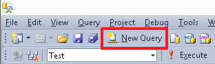
To create a new script editor, use the “New Query / New Query” button:



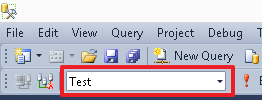
To change the current database, you can use the drop-down list:



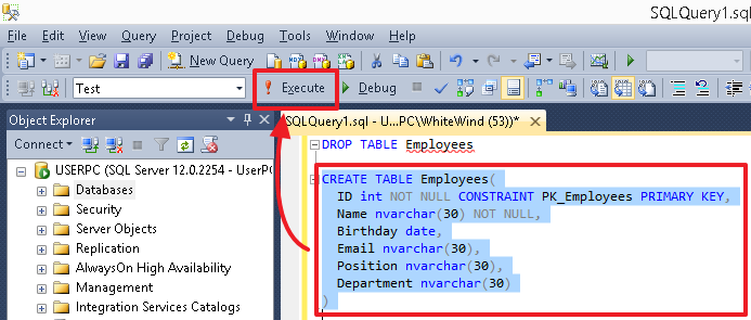
To execute a specific command (or group of commands), highlight it and press the “Execute / Execute” button or the F5 key. If there is only one command currently in the editor, or you need to execute all the commands, then you do not need to select anything.



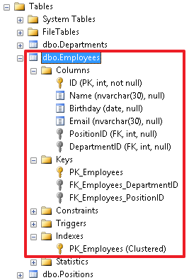
After executing scripts, in particular creating objects (tables, columns, indexes), to see the changes, use the update from the context menu, selecting the corresponding group (for example, Tables), the table itself or the Columns group in it.



Actually, this is all that we will need to know in order to carry out the examples cited here. The rest of the SSMS utility is easy to learn on your own.

Some theory

A relational database (DBD, or further in the context of simply DB) is a set of tables related to each other. Roughly speaking, a DB is a file in which data is stored in a structured form.

DBMS - Management System for these Databases, i.e. This is a set of tools for working with a specific type of database (MS SQL, Oracle, MySQL, Firebird, ...).

Note
Since in life, colloquially, we mostly say: “Oracle DB”, or even just “Oracle”, actually meaning “Oracle DBMS”, then the term DB will sometimes be used in the context of this textbook. From the context, I think it will be clear what exactly we are talking about.

A table is a collection of columns. Columns can also be called fields or columns, all these words will be used as synonyms expressing the same thing.

The table is the main object of the DDB, all DDB data is stored line by line in columns of the table. Lines, records are also synonyms.

For each table, as well as its columns, the names are set, which are subsequently referred to.
The name of an object (table name, column name, index name, etc.) in MS SQL can have a maximum length of 128 characters.

For reference , in the ORACLE database, object names can have a maximum length of 30 characters. Therefore, for a specific database, you need to develop your own rules for naming objects in order to meet the limit on the number of characters.

SQL is a language that allows queries in the database through the DBMS. In a specific DBMS, the SQL language can have a specific implementation (its own dialect).

DDL and DML is a subset of the SQL language:

• The DDL language serves to create and modify the database structure, i.e. to create / modify / delete tables and links.
• DML allows you to manipulate table data, i.e. with its strings. It allows you to make a selection of data from the tables, add new data to the table, as well as update and delete existing data.

In the SQL language, you can use 2 types of comments (single-line and multi-line):

--   

and

 /*   */ 

Actually, everything for the theory of this will be enough.

DDL - Data Definition Language

For example, consider a table with data about employees, in the usual form for a person who is not a programmer:

Personnel Number	Full name	Date of Birth	E-mail	Position	Department
1000	Ivanov I.I.	02/19/1955	i.ivanov@test.tt	Director	Administration
1001	Petrov P.P.	12/03/1983	p.petrov@test.tt	Programmer	IT
1002	Sidorov S.S.	06/07/1976	s.sidorov@test.tt	Accountant	Accounting
1003	Andreev A.A.	04/17/1982	a.andreev@test.tt	Senior programmer	IT

In this case, the columns of the table have the following names: Personnel number, full name, Date of birth, E-mail, Position, Department.

Each of these columns can be characterized by the type of data it contains:

• Personnel number - integer
• Name - string
• Date of birth - date
• E-mail - string
• Position - string
• Division - string

Column type is a characteristic that says what kind of data a given column can store.

For a start, it will be enough to remember only the following basic data types used in MS SQL:

Value	Designation in MS SQL	Description
Variable length string	varchar (N) and nvarchar (n)	Using the number N, we can specify the maximum possible row length for the corresponding column. For example, if we want to say that the value of the column "full name" can contain a maximum of 30 characters, then it is necessary to specify the type nvarchar (30). The difference between varchar and nvarchar is that varchar allows you to store strings in ASCII format, where one character takes 1 byte, and nvarchar stores strings in Unicode format, where each character takes 2 bytes. The varchar type should only be used if you are 100% sure that this field does not need to store Unicode characters. For example, varchar can be used to store email addresses, because they usually contain only ASCII characters.
Fixed length string	char (N) and nchar (N)	This type differs from a string of variable length in that if the length of the string is less than N characters, then it is always padded to the right to the length by N spaces and stored in the database in this form, that is in the database, it takes exactly N characters (where one character takes 1 byte for char and 2 bytes for type nchar). In my practice, this type is very rarely used, and if used, it is used mainly in the char (1) format, i.e. when a field is defined by a single character.
Integer	int	This type allows us to use only integers in the column, both positive and negative. For reference (now it is not so important for us) - the range of numbers that allows the int type from -2 147 483 648 to 2 147 483 647. Usually this is the main type that is used to set identifiers.
Real or real number	float	In simple terms, these are numbers in which a decimal point (comma) may be present.
date	date	If you need to store in the column only the Date, which consists of three components: Number, Month and Year. For example, February 15, 2014 (February 15, 2014). This type can be used for the column “Date of admission”, “Date of birth”, etc., i.e. when it is important for us to fix only the date, or when the time component is not important to us and it can be dropped or if it is not known.
Time	time	This type can be used if it is necessary to store only time data in the column, i.e. Hours, Minutes, Seconds and Milliseconds. For example, 17: 38: 31.3231603 For example, the daily flight departure time.
date and time	datetime	This type allows you to simultaneously save the date and time. For example, 02.15.2014 17: 38: 31.323 For example, this can be the date and time of an event.
Flag	bit	It is convenient to use this type for storing values ​​of the form “Yes” / “No”, where “Yes” will be stored as 1, and “No” will be stored as 0.

Also, the value of the field, in the event that this is not prohibited, may not be indicated, the keyword NULL is used for this purpose.

To execute the examples we will create a test database called Test.

A simple database (without additional parameters) can be created by running the following command:

 CREATE DATABASE Test 

You can delete a database with a command (you should be very careful with this command):

 DROP DATABASE Test 

In order to switch to our database, you can run the command:

 USE Test 

Or select the Test database in the drop-down list in the SSMS menu area. When I work, I often use this method of switching between databases.

Now in our database we can create a table using descriptions as they are, using spaces and Cyrillic characters:

 CREATE TABLE []( [ ] int, [] nvarchar(30), [ ] date, [E-mail] nvarchar(30), [] nvarchar(30), [] nvarchar(30) ) 

In this case, we will have to enclose the names in square brackets [...].

But in the database for greater convenience, all the names of the objects are better set in the Latin alphabet and not use spaces in the names. In MS SQL, usually in this case, each word begins with an uppercase letter, for example, for the field “Personnel number”, we could set the name PersonnelNumber. You can also use numbers in the name, for example, PhoneNumber1.

On a note
In some DBMS, the following format of the names “PHONE_NUMBER” may be more preferable, for example, such a format is often used in the ORACLE database. Naturally, when specifying the field name, it is desirable that it does not coincide with the keywords used in the DBMS.

For this reason, you can forget about the syntax with square brackets and delete the table [Employees]:

 DROP TABLE [] 

For example, a table with employees can be called “Employees”, and its fields can be given the following names:

• ID - Personnel number (Employee Identifier)
• Name - Full Name
• Birthday - Date of birth
• Email - E-mail
• Position - Position
• Department - Department

Very often the word ID is used to name the identifier field.

Now create our table:

 CREATE TABLE Employees( ID int, Name nvarchar(30), Birthday date, Email nvarchar(30), Position nvarchar(30), Department nvarchar(30) ) 

You can use the NOT NULL option to specify required columns.

For an existing table, fields can be overridden using the following commands:

 --   ID ALTER TABLE Employees ALTER COLUMN ID int NOT NULL --   Name ALTER TABLE Employees ALTER COLUMN Name nvarchar(30) NOT NULL 

On a note
The general concept of the SQL language for most DBMS remains the same (at least, I can judge this by the DBMS with which I happened to work). The difference in DDL in different DBMSs mainly lies in the data types (here not only their names can differ, but also the details of their implementation), the very specifics of the implementation of the SQL language can also differ slightly (i.e. the commands are the same, but there may be slight differences in the dialect, alas, but there is no one standard). Owning the basics of SQL, you can easily switch from one DBMS to another, because in this case, you only need to understand the implementation details of the commands in the new DBMS, i.e. in most cases it will be enough just to draw an analogy.

Not to be unfounded, I will give several examples of the same commands for the ORACLE DBMS:

 --   CREATE TABLE Employees( ID int, --  ORACLE  int -  ()  number(38) Name nvarchar2(30), -- nvarchar2  ORACLE  nvarchar  MS SQL Birthday date, Email nvarchar2(30), Position nvarchar2(30), Department nvarchar2(30) ); --   ID  Name (  ALTER COLUMN  MODIFY(…)) ALTER TABLE Employees MODIFY(ID int NOT NULL,Name nvarchar2(30) NOT NULL); --  PK (        MS SQL,    ) ALTER TABLE Employees ADD CONSTRAINT PK_Employees PRIMARY KEY(ID); 

For ORACLE there are differences in terms of implementation of the varchar2 type, its encoding depends on the database settings and the text can be saved, for example, in the UTF-8 encoding. In addition, the length of the field in ORACLE can be specified both in bytes and in characters; for this, additional options BYTE and CHAR are used, which are specified after the field length, for example:

 NAME varchar2(30 BYTE) --     30  NAME varchar2(30 CHAR) --     30  

Which option will be used by default BYTE or CHAR, in the case of a simple indication in ORACLE of type varchar2 (30), depends on the database settings, as it can sometimes be specified in the IDE settings. In general, sometimes you can easily get confused, so in the case of ORACLE, if the varchar2 type is used (and this is sometimes justified, for example, when using the UTF-8 encoding), I prefer to explicitly prescribe CHAR (because usually the string length is more convenient to read in characters ).

But in this case, if there is already any data in the table, then for the successful execution of commands it is necessary that the ID and Name fields in all rows of the table are necessarily filled. Let us demonstrate this with an example, insert data into the table in the ID, Position and Department fields, this can be done with the following script:

 INSERT Employees(ID,Position,Department) VALUES (1000,N'',N''), (1001,N'',N''), (1002,N'',N''), (1003,N' ',N'') 

In this case, the INSERT command will also generate an error, since when inserting, we did not specify the values ​​of the required Name field.
If we already had this data in the original table, then the “ALTER TABLE Employees ALTER COLUMN ID int NOT NULL” command would succeed, and the “ALTER TABLE Employees ALTER COLUMN Name int NOT NULL” command would generate an error message, that the Name field contains NULL (not specified) values.

Add values ​​for the Name field and fill the data again:

 INSERT Employees(ID,Position,Department,Name) VALUES (1000,N'',N'',N' ..'), (1001,N'',N'',N' ..'), (1002,N'',N'',N' ..'), (1003,N' ',N'',N' ..') 

Also, the NOT NULL option can be used directly when creating a new table, i.e. in the context of the CREATE TABLE command.

First, delete the table with the command:

 DROP TABLE Employees 

Now create a table with the required ID and Name columns:

 CREATE TABLE Employees( ID int NOT NULL, Name nvarchar(30) NOT NULL, Birthday date, Email nvarchar(30), Position nvarchar(30), Department nvarchar(30) ) 

You can also write NULL after the column name, which will mean that NULL values ​​(not specified) will be allowed in it, but this is not necessary, since this characteristic is implied by default.

If, on the contrary, it is necessary to make the existing column optional, then use the following command syntax:

 ALTER TABLE Employees ALTER COLUMN Name nvarchar(30) NULL 

Or simply:

 ALTER TABLE Employees ALTER COLUMN Name nvarchar(30) 

Also with this command we can change the field type to another compatible type, or change its length. For example, let's expand the Name field to 50 characters:

 ALTER TABLE Employees ALTER COLUMN Name nvarchar(50) 

Primary key

When creating a table, it is desirable that it have a unique column or a set of columns that is unique for each of its rows — you can uniquely identify a record by this unique value. This value is called the primary key of the table. For our Employees table, such a unique value can be an ID column (which contains the “Employee employee number” - let in our case this value is unique for each employee and cannot be repeated).

To create a primary key to an existing table, use the command:

 ALTER TABLE Employees ADD CONSTRAINT PK_Employees PRIMARY KEY(ID) 

Where “PK_Employees” is the name of the constraint responsible for the primary key. Usually for the name of the primary key is used the prefix "PK_" followed by the name of the table.

If the primary key consists of several fields, then these fields must be listed in brackets, separated by commas:

 ALTER TABLE _ ADD CONSTRAINT _ PRIMARY KEY(1,2,…) 

It should be noted that in MS SQL all fields that are included in the primary key must have the NOT NULL characteristic.

Also, the primary key can be determined directly when creating the table, i.e. in the context of the CREATE TABLE command. Delete the table:

 DROP TABLE Employees 

And then create it using the following syntax:

 CREATE TABLE Employees( ID int NOT NULL, Name nvarchar(30) NOT NULL, Birthday date, Email nvarchar(30), Position nvarchar(30), Department nvarchar(30), CONSTRAINT PK_Employees PRIMARY KEY(ID) --  PK   ,   ) 

After creating, fill in the data in the table:

 INSERT Employees(ID,Position,Department,Name) VALUES (1000,N'',N'',N' ..'), (1001,N'',N'',N' ..'), (1002,N'',N'',N' ..'), (1003,N' ',N'',N' ..') 

If the primary key in the table consists only of the values ​​of one column, then the following syntax can be used:

 CREATE TABLE Employees( ID int NOT NULL CONSTRAINT PK_Employees PRIMARY KEY, --     Name nvarchar(30) NOT NULL, Birthday date, Email nvarchar(30), Position nvarchar(30), Department nvarchar(30) ) 

In fact, the name of the restriction can be omitted, in which case it will be assigned a system name (like “PK__Employee__3214EC278DA42077”):

 CREATE TABLE Employees( ID int NOT NULL, Name nvarchar(30) NOT NULL, Birthday date, Email nvarchar(30), Position nvarchar(30), Department nvarchar(30), PRIMARY KEY(ID) ) 

Or:

 CREATE TABLE Employees( ID int NOT NULL PRIMARY KEY, Name nvarchar(30) NOT NULL, Birthday date, Email nvarchar(30), Position nvarchar(30), Department nvarchar(30) ) 

But I would recommend for permanent tables to always explicitly specify the name of the constraint, since by an explicitly given and understandable name, it will later be easier to manipulate it, for example, you can delete it:

 ALTER TABLE Employees DROP CONSTRAINT PK_Employees 

But such a short syntax, without specifying constraint names, is convenient to use when creating temporary database tables (the name of the temporary table starts with # or ##), which will be deleted after use.

Summarize

At the moment we have considered the following commands:

• CREATE TABLE table_name (enumeration of fields and their types, restrictions) - serves to create a new table in the current database;
• DROP TABLE table_name - serves to delete a table from the current database;
• ALTER TABLE tbl_name ALTER COLUMN col_name_name ... - used to update the column type or change its settings (for example, to set the NULL or NOT NULL characteristic);
• ALTER TABLE tbl_name ADD CONSTRAINT constraint_name PRIMARY KEY (field1, field2, ...) - add a primary key to an existing table;
• ALTER TABLE tbl_name DROP CONSTRAINT constraint-name - remove a constraint from a table.

It is a little about temporary tables

Cut from MSDN. In MS SQL Server, there are two types of temporary tables: local (#) and global (##). Local temporary tables are visible only to their creators until the end of the session to connect to the instance of SQL Server, as soon as they are first created. Local temporary tables are automatically deleted after the user is disconnected from the instance of SQL Server. Global temporary tables are visible to all users during any connection sessions after creating these tables and are deleted when all users referring to these tables are disconnected from the instance of SQL Server.

Temporary tables are created in the tempdb system database, i.e. creating them, we do not litter the main database, otherwise the temporary tables are completely identical to regular tables, they can also be deleted using the DROP TABLE command. Local (#) temporary tables are most commonly used.

To create a temporary table, you can use the CREATE TABLE command:

 CREATE TABLE #Temp( ID int, Name nvarchar(30) ) 

Since the temporary table in MS SQL is similar to a regular table, it can also be deleted by the DROP TABLE command itself:

 DROP TABLE #Temp 

You can also create a temporary table (like a regular table itself) and immediately fill it with data returned by the query using the SELECT ... INTO syntax:

 SELECT ID,Name INTO #Temp FROM Employees 

On a note
In different DBMS, the implementation of temporary tables may differ. For example, in ORACLE and Firebird DBMS, the structure of temporary tables should be defined in advance by the CREATE GLOBAL TEMPORARY TABLE command specifying the specifics of data storage in it, then the user can see it among the main tables and work with it as with a regular table.

Normalization of a DB - crushing on subtables (reference books) and definition of communications

Our current Employees table has the disadvantage that the user can enter any text in the Position and Department fields, which is fraught with errors first of all, since one employee can simply specify “IT” as a department, and the second employee, for example , enter the "IT department", the third "IT". As a result, it will be unclear what the user meant, i.e. Are these employees employees of the same department, or is the user described and these are 3 different departments? And even more so, in this case, we will not be able to correctly group the data for a report, where, it may be necessary to show the number of employees in the context of each department.

The second drawback is the storage volume of this information and its duplication, i.e. For each employee, the full name of the department is indicated, which requires a place in the database to store each character from the department name.

The third drawback is the difficulty of updating these fields, if the name of a post changes, for example, if you need to rename the post “Programmer” to “Junior Programmer”. In this case, we will have to make changes to every line of the table for which the Position is equal to "Programmer".

To avoid these shortcomings, the so-called database normalization is applied - splitting it into subtables, tables of reference books. It is not necessary to climb into the wilds of the theory and study what normal forms are, it is enough to understand the essence of normalization.

Let's create 2 tables of references “Posts” and “Departments”, the first one will be called Positions, and the second one, respectively, Departments:

 CREATE TABLE Positions( ID int IDENTITY(1,1) NOT NULL CONSTRAINT PK_Positions PRIMARY KEY, Name nvarchar(30) NOT NULL ) CREATE TABLE Departments( ID int IDENTITY(1,1) NOT NULL CONSTRAINT PK_Departments PRIMARY KEY, Name nvarchar(30) NOT NULL ) 

Note that here we used the new IDENTITY option, which says that the data in the ID column will be numbered automatically, starting with 1, with step 1, i.e. when new records are added, they will be sequentially assigned the values ​​1, 2, 3, etc. Such fields are usually called auto-increment. Only one field with the IDENTITY property can be defined in a table and usually, but not necessarily, such a field is the primary key for this table.

On a note
In different DBMS, the implementation of fields with a counter can be done in its own way. In MySQL, for example, such a field is defined using the AUTO_INCREMENT option. In ORACLE and Firebird, this functionality could previously be emulated using sequence (SEQUENCE). But as far as I know in ORACLE now added option GENERATED AS IDENTITY.

Let's fill these tables automatically, based on the current data recorded in the Position and Department fields of the Employees table:

 --   Name  Positions,     Position  Employees INSERT Positions(Name) SELECT DISTINCT Position FROM Employees WHERE Position IS NOT NULL --        

Do the same for the Departments table:

 INSERT Departments(Name) SELECT DISTINCT Department FROM Employees WHERE Department IS NOT NULL 

If we now open the Positions and Departments tables, we see a numbered set of values ​​across the ID field:

 SELECT * FROM Positions 

ID	Name
one	Accountant
2	Director
3	Programmer
four	Senior programmer

 SELECT * FROM Departments 

ID	Name
one	Administration
2	Accounting
3	IT

These tables now will play the role of reference books for the assignment of posts and departments. Now we will refer to the identifiers of posts and departments. First of all, create new fields in the Employees table for storing identifier data:

 --    ID  ALTER TABLE Employees ADD PositionID int --    ID  ALTER TABLE Employees ADD DepartmentID int 

The type of the reference fields must be what, as in the reference books, in this case it is an int.

You can also add several fields to the table at once with one command, listing the fields separated by commas:

 ALTER TABLE Employees ADD PositionID int, DepartmentID int 

Now we will write the links (reference constraints - FOREIGN KEY) for these fields, so that the user does not have the opportunity to write in these fields, values ​​that are missing among the ID values ​​in the reference books.

 ALTER TABLE Employees ADD CONSTRAINT FK_Employees_PositionID FOREIGN KEY(PositionID) REFERENCES Positions(ID) 

And we will do the same for the second field:

 ALTER TABLE Employees ADD CONSTRAINT FK_Employees_DepartmentID FOREIGN KEY(DepartmentID) REFERENCES Departments(ID) 

Now the user can enter only the ID values ​​from the corresponding directory in these fields. Accordingly, in order to use a new department or position, it must first add a new entry to the appropriate directory. Sinceposts and departments are now stored in reference books in one single copy, then in order to change the name, it is enough to change it only in the reference book.

The name of the reference constraint is usually composite, it consists of the “FK_” prefix, then the name of the table and, after the underscore, the name of the field that refers to the identifier of the reference table.

The identifier (ID) is usually an internal value that is used only for links and what value is stored there, in most cases absolutely indifferent, so you should not try to get rid of holes in the sequence of numbers that occur during the work with the table, for example, after deleting records from the directory.

Also, in some cases, the link can be organized in several fields:

 ALTER TABLE  ADD CONSTRAINT _ FOREIGN KEY(1,2,…) REFERENCES _(1,2,…) 

In this case, in the table "reference_ table", the primary key is represented by a combination of several fields (field1, field2, ...).

Actually, we now update the PositionID and DepartmentID fields with ID values ​​from reference books. For this purpose, we use the DML UPDATE command:

 UPDATE e SET PositionID=(SELECT ID FROM Positions WHERE Name=e.Position), DepartmentID=(SELECT ID FROM Departments WHERE Name=e.Department) FROM Employees e 

Let's see what happened by running the query:

 SELECT * FROM Employees 

ID	Name	Birthday	Email	Position	Department	PositionID	DepartmentID
1000	Ivanov I.I.	Null	Null	Director	Administration	2	one
1001	Petrov P.P.	Null	Null	Programmer	IT	3	3
1002	Sidorov S.S.	Null	Null	Accountant	Accounting	one	2
1003	Andreev A.A.	Null	Null	Senior programmer	IT	four	3

Everything, the PositionID and DepartmentID fields are filled with the corresponding positions and departments with identifiers of need for the Position and Department fields in the Employees table now no, you can delete these fields:

 ALTER TABLE Employees DROP COLUMN Position,Department 

Now the table has acquired the following form:

 SELECT * FROM Employees 

ID	Name	Birthday	Email	PositionID	DepartmentID
1000	Ivanov I.I.	Null	Null	2	one
1001	Petrov P.P.	Null	Null	3	3
1002	Sidorov S.S.	Null	Null	one	2
1003	Andreev A.A.	Null	Null	four	3

Those.we eventually got rid of storing redundant information. Now, by the position and department numbers we can uniquely identify their names using the values ​​in the reference tables:

 SELECT e.ID,e.Name,p.Name PositionName,d.Name DepartmentName FROM Employees e LEFT JOIN Departments d ON d.ID=e.DepartmentID LEFT JOIN Positions p ON p.ID=e.PositionID 

ID	Name	PositionName	DepartmentName
1000	Ivanov I.I.	Director	Administration
1001	..	Programmer	IT
1002	..	Accountant	Accounting
1003	..	Senior programmer	IT

, . – , .



, , .. . ManagerID, , . :

 ALTER TABLE Employees ADD ManagerID int 

NULL, , , , .

FOREIGN KEY Employees:

 ALTER TABLE Employees ADD CONSTRAINT FK_Employees_ManagerID FOREIGN KEY (ManagerID) REFERENCES Employees(ID) 

Let's now create a diagram and see how the links between our tables look on it:





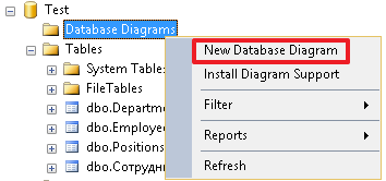
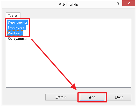
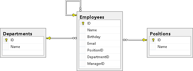
As a result, we should see the following picture (the Employees table is associated with the Positions and Depertments tables, and also refers to itself):



Finally, we should say that reference keys may include additional options ON DELETE CASCADE and ON UPDATE CASCADE, which talk about how to behave when deleting or updating a record referenced in the reference table. If these options are not specified, then we cannot change the ID in the table of the reference book of the entry referenced from another table, nor can we delete such entry from the reference book until we delete all the rows referring to this entry or we will update in these lines links to another value.

ON DELETE CASCADE FK_Employees_DepartmentID:

 DROP TABLE Employees CREATE TABLE Employees( ID int NOT NULL, Name nvarchar(30), Birthday date, Email nvarchar(30), PositionID int, DepartmentID int, ManagerID int, CONSTRAINT PK_Employees PRIMARY KEY (ID), CONSTRAINT FK_Employees_DepartmentID FOREIGN KEY(DepartmentID) REFERENCES Departments(ID) ON DELETE CASCADE, CONSTRAINT FK_Employees_PositionID FOREIGN KEY(PositionID) REFERENCES Positions(ID), CONSTRAINT FK_Employees_ManagerID FOREIGN KEY (ManagerID) REFERENCES Employees(ID) ) INSERT Employees (ID,Name,Birthday,PositionID,DepartmentID,ManagerID)VALUES (1000,N' ..','19550219',2,1,NULL), (1001,N' ..','19831203',3,3,1003), (1002,N' ..','19760607',1,2,1000), (1003,N' ..','19820417',4,3,1000) 

3 Departments:

 DELETE Departments WHERE ID=3 

Employees:

 SELECT * FROM Employees 

ID	Name	Birthday	Email	PositionID	DepartmentID	ManagerID
1000	Ivanov I.I.	1955-02-19	Null	2	one	Null
1002	..	1976-06-07	Null	one	2	1000

, 3 Employees .

ON UPDATE CASCADE , ID . , ID , DepartmentID Employees ID . , .. ID Departments IDENTITY, ( 3 30):

 UPDATE Departments SET ID=30 WHERE ID=3 

The main thing to understand the essence of these 2 options ON DELETE CASCADE and ON UPDATE CASCADE. I use these options very rarely and I recommend that you think carefully before specifying them in the reference constraint, since in case of unintentional deletion of a record from the reference table, this can lead to big problems and create a chain reaction.

Restore section 3:

 --    / IDENTITY  SET IDENTITY_INSERT Departments ON INSERT Departments(ID,Name) VALUES(3,N'') --  / IDENTITY  SET IDENTITY_INSERT Departments OFF 

Completely clear the Employees table using the TRUNCATE TABLE command:

 TRUNCATE TABLE Employees 

Again, let's reload the data into it using the previous INSERT command:

 INSERT Employees (ID,Name,Birthday,PositionID,DepartmentID,ManagerID)VALUES (1000,N' ..','19550219',2,1,NULL), (1001,N' ..','19831203',3,3,1003), (1002,N' ..','19760607',1,2,1000), (1003,N' ..','19820417',4,3,1000) 

Summarize

At this point, a few more DDL commands have been added to our knowledge:

• Adding the IDENTITY property to the field - allows you to make this field automatically populated (by a counter field) for the table;
• ALTER TABLE tbl_name ADD list_fields_characteristics - allows you to add new fields to the table;
• ALTER TABLE _ DROP COLUMN _ – ;
• ALTER TABLE _ ADD CONSTRAINT _ FOREIGN KEY () REFERENCES _() – .

– UNIQUE, DEFAULT, CHECK

UNIQUE . Employees, Email. Email , :

 UPDATE Employees SET Email='i.ivanov@test.tt' WHERE ID=1000 UPDATE Employees SET Email='p.petrov@test.tt' WHERE ID=1001 UPDATE Employees SET Email='s.sidorov@test.tt' WHERE ID=1002 UPDATE Employees SET Email='a.andreev@test.tt' WHERE ID=1003 

-:

 ALTER TABLE Employees ADD CONSTRAINT UQ_Employees_Email UNIQUE(Email) 

Now the user will not be able to enter the same E-Mail with several employees.

The uniqueness restriction is usually referred to as follows - first comes the prefix “UQ_”, then the name of the table and after the underscore sign the name of the field on which this restriction is imposed.

Accordingly, if the combination of fields should be unique in the context of table rows, we list them separated by commas:

 ALTER TABLE _ ADD CONSTRAINT _ UNIQUE(1,2,…) 

DEFAULT , , INSERT. .

Employees « » HireDate :

 ALTER TABLE Employees ADD HireDate date NOT NULL DEFAULT SYSDATETIME() 

HireDate , :

 ALTER TABLE Employees ADD DEFAULT SYSDATETIME() FOR HireDate 

, .. DEFAULT , . -, , , . This is done as follows:

 ALTER TABLE Employees ADD CONSTRAINT DF_Employees_HireDate DEFAULT SYSDATETIME() FOR HireDate 

Since this column was not there before, then when it is added to each record, the current date value will be inserted in the HireDate field.

When adding a new record, the current date will also be inserted automatically, of course, unless we explicitly specify it, i.e. do not specify in the list of columns. Let us show this with an example, without specifying the HireDate field in the list of added values:

 INSERT Employees(ID,Name,Email)VALUES(1004,N' ..','s.sergeev@test.tt') 

Let's see what happened:

 SELECT * FROM Employees 

ID	Name	Birthday	Email	PositionID	DepartmentID	ManagerID	Hiredate
1000	Ivanov I.I.	1955-02-19	i.ivanov@test.tt	2	one	Null	2015-04-08
1001	Petrov P.P.	1983-12-03	p.petrov@test.tt	3	four	1003	2015-04-08
1002	Sidorov S.S.	1976-06-07	s.sidorov@test.tt	one	2	1000	2015-04-08
1003	Andreev A.A.	1982-04-17	a.andreev@test.tt	four	3	1000	2015-04-08
1004	Sergeev S.S.	Null	s.sergeev@test.tt	Null	Null	Null	2015-04-08

The check constraint CHECK is used when it is necessary to check the values ​​inserted in the field. For example, we impose this restriction on the field of personnel number, which we have is an employee identifier (ID). Using this restriction, we say that personnel numbers should have a value from 1000 to 1999:

 ALTER TABLE Employees ADD CONSTRAINT CK_Employees_ID CHECK(ID BETWEEN 1000 AND 1999) 

The constraint is usually named the same, first comes the prefix “CK_”, then the name of the table and the name of the field on which this restriction is imposed.

Let's try inserting an invalid entry to verify that the constraint is working (we should get the corresponding error):

 INSERT Employees(ID,Email) VALUES(2000,'test@test.tt') 

And now we change the inserted value to 1500 and make sure that the record is inserted:

 INSERT Employees(ID,Email) VALUES(1500,'test@test.tt') 

You can also create UNIQUE and CHECK constraints without specifying a name:

 ALTER TABLE Employees ADD UNIQUE(Email) ALTER TABLE Employees ADD CHECK(ID BETWEEN 1000 AND 1999) 

But this is not very good practice and it is better to set the name of the constraint explicitly, since in order to understand later what will be more difficult, it will be necessary to open the object and look at what it is responsible for.



With a good name a lot of information about the restriction can be found directly by its name.

And, accordingly, all these restrictions can be created immediately when creating a table, if it does not already exist. Delete the table:

 DROP TABLE Employees 

And we will recreate it with all created restrictions with a single CREATE TABLE command:

 CREATE TABLE Employees( ID int NOT NULL, Name nvarchar(30), Birthday date, Email nvarchar(30), PositionID int, DepartmentID int, HireDate date NOT NULL DEFAULT SYSDATETIME(), --  DEFAULT    CONSTRAINT PK_Employees PRIMARY KEY (ID), CONSTRAINT FK_Employees_DepartmentID FOREIGN KEY(DepartmentID) REFERENCES Departments(ID), CONSTRAINT FK_Employees_PositionID FOREIGN KEY(PositionID) REFERENCES Positions(ID), CONSTRAINT UQ_Employees_Email UNIQUE (Email), CONSTRAINT CK_Employees_ID CHECK (ID BETWEEN 1000 AND 1999) ) 

Finally, insert our employees into the table:

 INSERT Employees (ID,Name,Birthday,Email,PositionID,DepartmentID)VALUES (1000,N' ..','19550219','i.ivanov@test.tt',2,1), (1001,N' ..','19831203','p.petrov@test.tt',3,3), (1002,N' ..','19760607','s.sidorov@test.tt',1,2), (1003,N' ..','19820417','a.andreev@test.tt',4,3) 

It is a little about the indexes created at creation of restrictions PRIMARY KEY and UNIQUE

, PRIMARY KEY UNIQUE (PK_Employees UQ_Employees_Email). CLUSTERED, NONCLUSTERED. , . (CLUSTERED) . CLUSTERED – , , , . . , , . – , , . , , , NONCLUSTERED:

 ALTER TABLE _ ADD CONSTRAINT _ PRIMARY KEY NONCLUSTERED(1,2,…) 

For example, let's make the restriction index PK_Employees noncluster, and the restriction index UQ_Employees_Email cluster. First, remove these restrictions:

 ALTER TABLE Employees DROP CONSTRAINT PK_Employees ALTER TABLE Employees DROP CONSTRAINT UQ_Employees_Email 

Now create them with the CLUSTERED and NONCLUSTERED options:

 ALTER TABLE Employees ADD CONSTRAINT PK_Employees PRIMARY KEY NONCLUSTERED (ID) ALTER TABLE Employees ADD CONSTRAINT UQ_Employees_Email UNIQUE CLUSTERED (Email) 

Now, selecting the Employees table, we see that the records were sorted by the cluster index UQ_Employees_Email:

 SELECT * FROM Employees 

ID	Name	Birthday	Email	PositionID	DepartmentID	Hiredate
1003	Andreev A.A.	1982-04-17	a.andreev@test.tt	four	3	2015-04-08
1000	Ivanov I.I.	1955-02-19	i.ivanov@test.tt	2	one	2015-04-08
1001	Petrov P.P.	1983-12-03	p.petrov@test.tt	3	3	2015-04-08
1002	Sidorov S.S.	1976-06-07	s.sidorov@test.tt	one	2	2015-04-08

Prior to this, when the cluster index was the PK_Employees index, the default entries were sorted by the ID field.

But in this case, this is just an example that shows the essence of the cluster index, since Most likely, queries on the ID field will be made to the Employees table and in some cases, it will probably act as a directory itself.

For directories, it is usually advisable that the cluster index be built on the primary key, since in queries, we often refer to a directory identifier for obtaining, for example, a name (Position, Department). Here we recall what I wrote above that the cluster index has direct access to the rows of the table, and it follows that we can get the value of any column without additional overhead.

Cluster index is advantageous to apply to the fields in which the sample is most often.

Sometimes, in tables, a key is created for a surrogate field, in this case it is useful to save the CLUSTERED index option for a more suitable index and specify the NONCLUSTERED option when creating a surrogate primary key.

Summarize

At this stage, we got acquainted with all kinds of restrictions, in their simplest form, which are created by a command like "ALTER TABLE tablename ADD CONSTRAINT name_ restrictions ...":

• PRIMARY KEY - primary key;
• FOREIGN KEY - setting up links and monitoring referential integrity of data;
• UNIQUE - allows you to create uniqueness;
• CHECK - allows the correctness of the entered data;
• DEFAULT - allows you to set a default value;
• It is also worth noting that all restrictions can be removed using the command « the ALTER TABLE statement table_name DROP CONSTRAINT constraint_name".

We also partially covered the topic of indexes and dismantled the concept of cluster ( CLUSTERED ) and non-cluster ( NONCLUSTERED ) index.

Creation of independent indexes

Independence here refers to indices that are not created to restrict PRIMARY KEY or UNIQUE.

Indexes by field or fields can be created with the following command:

 CREATE INDEX IDX_Employees_Name ON Employees(Name) 

Here you can also specify the CLUSTERED, NONCLUSTERED, UNIQUE options, as well as the sort direction for each individual ASC field (default) or DESC:

 CREATE UNIQUE NONCLUSTERED INDEX UQ_Employees_EmailDesc ON Employees(Email DESC) 

NONCLUSTERED , .. , , CLUSTERED NONCLUSTERED .

:

 DROP INDEX IDX_Employees_Name ON Employees 

, , CREATE TABLE.

:

 DROP TABLE Employees 

CREATE TABLE:

 CREATE TABLE Employees( ID int NOT NULL, Name nvarchar(30), Birthday date, Email nvarchar(30), PositionID int, DepartmentID int, HireDate date NOT NULL CONSTRAINT DF_Employees_HireDate DEFAULT SYSDATETIME(), ManagerID int, CONSTRAINT PK_Employees PRIMARY KEY (ID), CONSTRAINT FK_Employees_DepartmentID FOREIGN KEY(DepartmentID) REFERENCES Departments(ID), CONSTRAINT FK_Employees_PositionID FOREIGN KEY(PositionID) REFERENCES Positions(ID), CONSTRAINT FK_Employees_ManagerID FOREIGN KEY (ManagerID) REFERENCES Employees(ID), CONSTRAINT UQ_Employees_Email UNIQUE(Email), CONSTRAINT CK_Employees_ID CHECK(ID BETWEEN 1000 AND 1999), INDEX IDX_Employees_Name(Name) ) 

:

 INSERT Employees (ID,Name,Birthday,Email,PositionID,DepartmentID,ManagerID)VALUES (1000,N' ..','19550219','i.ivanov@test.tt',2,1,NULL), (1001,N' ..','19831203','p.petrov@test.tt',3,3,1003), (1002,N' ..','19760607','s.sidorov@test.tt',1,2,1000), (1003,N' ..','19820417','a.andreev@test.tt',4,3,1000) 

, INCLUDE. Those. INCLUDE- - , , . , (SELECT), , . , .. .

MSDN.

 CREATE [ UNIQUE ] [ CLUSTERED | NONCLUSTERED ] INDEX index_name ON <object> ( column [ ASC | DESC ] [ ,...n ] ) [ INCLUDE ( column_name [ ,...n ] ) ] 

Summarize

(SELECT), , .. .

, , , . , , .

DDL

, DDL , . , .

— , .

SQL.

Part Two - habrahabr.ru/post/255523