Simulate sensor readings using an array of waypoints

Publication structure

• Roll forward clause
• Preparing a GPS track
• How to get Krylov-Euler angles from an array of vectors
• Imitation of gyroscope readings
• The vector of acceleration of gravity and the direction of "north"
• Simulation of accelerometer, compass and barometer readings

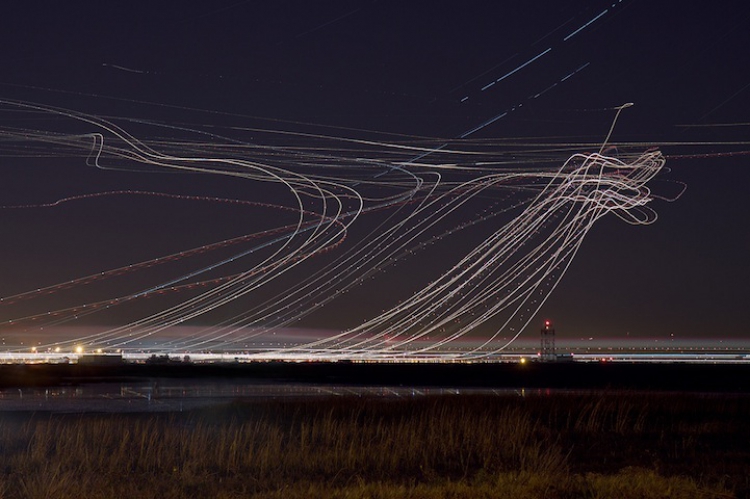
To debug the algorithm, working with inertial navigation sensors, you may need to simulate the readings of these sensors. For example, you have a debugging sequence of waypoints simulating a certain situation. You can have some kind of GPS-track, which has features, or not having them. In my case, there is a field test result, but the board is not ready yet (in production) - you need to do something.

')

Roll forward clause

It should be immediately noted that when moving, the 3D point does not give us information about the position of the body relative to the axis of movement. If we imagine that a thread is stretched between the points of the path, and our object is a bead, then it will move along the thread clearly, and can rotate freely around the axis of motion. As the direction of motion we will use the velocity vector and we will remember the reservation about the roll in the result.

Preparing a GPS track

If you have a GPS track as source data, you need to first prepare it. It is required to convert the existing file to a format from which data can be obtained. I converted to GPX (since inside it is XML).

<trkpt lat="12.345678" lon="87.654321"> <ele>839</ele> <time>2013-05-09T11:24:28.776Z</time> <extensions> <mytracks c="194.9" s="9.25" /> </extensions> </trkpt> . . . <trkpt lat="12.345678" lon="87.654321"> <ele>837</ele> <time>2013-05-09T11:24:31.779Z</time> <extensions> <mytracks c="195.7" s="8.68" /> </extensions> </trkpt> 

Next, we take any available database (for example, MySQL), create a label and fill it with data from the received XML. The XML format may be different - the main thing is to find the latitude, longitude, altitude and time. We create the first label, for example 'xml_src'. All columns for ease of loading do string.



Let's get some data. For convenience, create a second table, for example, 'points'. MySQL code:

 insert into points (lat,lon,h,dt) SELECT cast(xx.lat AS DECIMAL(11, 6)) , cast(xx.lon AS DECIMAL(11, 6)) , cast(xx.ele AS DECIMAL(11, 6)) , cast(replace(replace(xx.`time`, "T", " "), "Z", "") AS DATETIME) FROM xml_src AS xx; 

As a result, we have the following:


Then we translate latitude and longitude into meters (see the article “Entertaining Geodesy” or use database tools, for example, in MSSQL, see the ShortestLineTo method). Convert to meters as follows. We assume that the coordinates of the first point are X = 0, Y = 0. The coordinates of each subsequent point are relative to the first one. We determine the distance between the points, first vertically, then horizontally in meters. The function for calculating the distance is in the article “Determining the distance between geographic points in MySQL” .



We translate the time in seconds so that the first line has 0 seconds (just subtract the value of the first line from the rest).


As a result, we have the following:


Now we need to get the coordinates of the point at regular intervals. The fact that the second point appeared 4 seconds after the first, the third after 2 seconds, and the next after a second does not suit us so much. Are we going to imitate the sensors? And they measure values ​​at equal intervals of time.

To obtain the coordinates of a point at regular intervals, we use interpolation. As an interpolation tool we use a one-dimensional cubic spline . I had Excel at hand, I wrote a macro in it (see spoiler). At this stage we decide with what frequency each “sensor” will work. For example, all “sensors” will give values ​​10 times per second. That is, the interval between measurements is 0.1 seconds.

Interpolate in pairs:

1. Time is X
2. Time - Y
3. Time - Z

The result is a table with the coordinates of the points of the “object” in which our “sensors” are located. The time interval between points is 0.1 seconds. The time of appearance of the coordinates of a particular point is calculated by the formula t = n / 10, where n is the line number.

How to get Krylov-Euler angles from an array of vectors

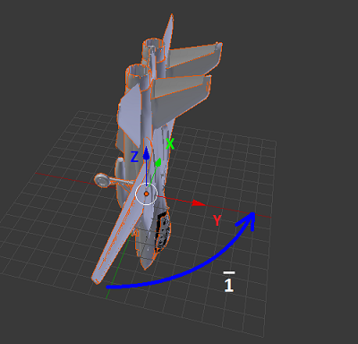
Take the movement of the nose of the aircraft from my previous article :




The coordinates of the point meaning the nose are equal:


Let's define all three turns. To do this, we obtain the axis of the first rotation v and the angle of the first rotation alf around the axis. Let the points of the path are the vertices of the vectors. Then the axis is obtained by multiplying the neighboring vectors.

v12 = v1 * v2 = (1; 0; 0) * (0; 1; 0) = (0; 0; 1)

The angle is calculated as follows:

 Public Function vectors_angle(v1 As TVector, v2 As TVector) As Double v1 = normal(v1) v2 = normal(v2) vectors_angle = Application.WorksheetFunction.Acos(v1.x * v2.x + v1.y * v2.y + v1.z * v2.z) End Function 

Alf12 = 90. Now create a quaternion based on the resulting axes and angles:

 Public Function create_quat(rotate_vector As TVector, rotate_angle As Double) As TQuat rotate_vector = normal(rotate_vector) create_quat.w = Cos(rotate_angle / 2) create_quat.x = rotate_vector.x * Sin(rotate_angle / 2) create_quat.y = rotate_vector.y * Sin(rotate_angle / 2) create_quat.z = rotate_vector.z * Sin(rotate_angle / 2) End Function 

We get the first quaternion:

(w = 0.7071; x = 0; y = 0; z = 0.7071)

From the quaternion we get the rotation components:

  sqw = w * w sqx = x * x sqy = y * y sqz = z * z bank = atan2(2 * (w * x + y * z), 1 - 2 * (sqx + sqy)) altitude = Application.WorksheetFunction.Asin(2 * (w * y - x * z)) heading = atan2(2 * (w * z + x * y), 1 - 2 * (sqy + sqz)) 

The result of determining the first turn: course = 90, pitch = 0, roll = 0.

We cannot calculate the remaining turns, because after the first turn, the local coordinate system of the aircraft no longer coincides with the global coordinate system. To determine the second turn from the position of the nose of the aircraft No. 2 to the position No. 3, you must first cancel the first turn, that is, return the reporting system to the place and with it unfold a new resultant vector. This requires obtaining the inverse quaternion of the first reversal and applying it to vectors №2 and №3 (obtaining the inverse quaternion and rotating the vector by the quaternion - see the article ).
Reverse quaternion of the first turn (rotation counterclockwise along the Z axis):

(w = 0.7071; x = 0; y = 0; z = -0.7071)

After applying this quaternion, the second and third vectors are equal:
v2 = (x = 1; y = 0; z = 0)
v3 = (x = 0; y = 0; z = -1)



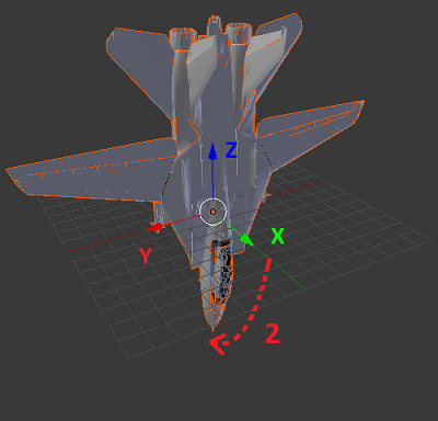
When the local coordinate system is aligned with the global one, it is possible to calculate the second quaternion and the components of the second rotation as described above:

(w = 0.7071; x = 0; y = 0; z = -0.7071),
course = 0, pitch = 90, roll = 0.

Next, we must memorize the perfect turns in the local coordinate system. To do this, we will create a separate quaternion and multiply the quaternions of turns into it:


Then from the quaternion of the series of perfect turns we will receive the inverse quaternion for combining the reporting systems.

Summarize. To get the components of the turns on the list of vectors that indicate the direction of motion, you need to do the following:

 '  " " q_mul.w = 1 q_mul.x = 0 q_mul.y = 0 q_mul.z = 0 For row_n = M To N '     v1.x = Application.ActiveWorkbook.ActiveSheet.Cells(row_n - 1, 1).Value v1.y = Application.ActiveWorkbook.ActiveSheet.Cells(row_n - 1, 2).Value v1.z = Application.ActiveWorkbook.ActiveSheet.Cells(row_n - 1, 3).Value '     v2.x = Application.ActiveWorkbook.ActiveSheet.Cells(row_n, 1).Value v2.y = Application.ActiveWorkbook.ActiveSheet.Cells(row_n, 2).Value v2.z = Application.ActiveWorkbook.ActiveSheet.Cells(row_n, 3).Value '        q_inv = myMath.quat_invert(q_mul) '    v1 = myMath.quat_transform_vector(q_inv, v1) '    '        (length(v1); 0; 0) –    v2 = myMath.quat_transform_vector(q_inv, v2) '    '     r12 = myMath.vecmul(v1, v2) '   alf = myMath.vectors_angle(v1, v2) '     q12 = myMath.create_quat(r12, alf) '         '    ypr = myMath.quat_to_krylov(q12) Application.ActiveWorkbook.ActiveSheet.Cells(row_n, 4).Value = ypr.heading Application.ActiveWorkbook.ActiveSheet.Cells(row_n, 5).Value = ypr.altitude Application.ActiveWorkbook.ActiveSheet.Cells(row_n, 6).Value = ypr.bank '     q_mul = myMath.quat_mul_quat(q_mul, q12) '   Next 

In this macro for Excel, the vectors are read from the first three bars. The result is written in 4, 5, 6 column.

Imitation of gyroscope readings

As you understand, the coordinates of the points are not suitable as input data - we need velocity vectors.

It is easy to get speed and acceleration from the prepared data - the difference between the adjacent lines of the point coordinates table is the speed, the difference between the adjacent speed lines is the acceleration. Just need to remember about the frequency of measurements. In this case, we have 10 "measurements" per second. This means that in order to get, for example, the speed in meters per second, you need to multiply the value of the corresponding cell by 10.



Take the velocity vectors and get the rotation components.



Now about the gyroscope. Gyro shows angular velocity. Our components of turns in the local coordinate system at equal intervals of time - this is the angular velocity.

In addition to obtaining the angular velocity, you need to add more noise. There are two tangible components in the gyroscope noise - the sensor's own noise (uniform distribution) and the effect of the earth's rotation (if your “sensor” is not in space). The intrinsic noise level of the sensor is described in the specification (we study the datasheet on the simulated sensor). My sensor has a resolution of 16 bits and has 4 measurement modes. Each mode has its maximum: the first one has ± 250º / sec, ... the fourth one has ± 2000º / sec. Sensitivity for the first mode 131 LSB / (º / s). To calculate this in degrees, you need to use the formula:

Sensitivity = Sensitivity_LSB * Maximum / Resolution = 131 * ± 250 / (2 ^ 16) = 131 * ± 250/65536 = ± 0.49972534 º / sec.

That is, the magnitude of the noise within one degree. Formula for Excel:
= (RIP () - 0.5) / N, where N is the number of simulated "measurements" per second.

The earth rotates at a speed of 15 degrees per hour. This is 0.0041667 degrees per second, which is much less than the measurement error. For fun, you can calculate it.

Suppose that the axis of rotation of the Earth coincides with the axis Z. Suppose also that the body is at the equator and the axis Y of the body is oriented strictly to the north (tangential). Then the axis X of the body coincides with the tangent direction of rotation. In this case, the axis of rotation of the Earth and the body along with it coincides with the axis Z of the body. Let us visualize the displacement in the latitude of our body to the north. Then the axis of rotation will rotate around the X axis clockwise by a number of degrees equal to the value of the new latitude. When shifting to the northern hemisphere, it is a plus sign, to the southern one, it is a minus sign. When the body is freely oriented in space, the free fall acceleration vector g will help us.



To calculate the axis of rotation of the Earth in the local coordinate system, you need:

1. Multiply the vector g by the vector of the compass reading "north".
2. Create a quaternion based on the resulting vector and angle. We take latitude as the angle value.
3. Expand the resulting quaternion vector compass "to the north."

To obtain the values ​​of the rotation of our body by the planet at the time of each measurement we do:

1. We calculate the vector of the axis of rotation of the planet using the current latitude from the source data.
2. Calculate how much the planet has turned since the last measurement. In our case, when measured 10 times per second, it will be 0.0041667 / 10 = 0.00041667.
3. We build a quaternion on the basis of the axis vector and the rotation angle.
4. We get the three components of the reversal (course, pitch, roll) and add to the readings of the “sensor”.

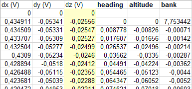
In general, as a result, we get the table:


The last three columns are “gyro readings”.

The vector of acceleration of gravity and the direction of "north"

Suppose that there is a unit vector C, which coincides with the tangent to the meridian and the direction "south" -> "north". Let the Y axis of our global coordinate system coincides with the vector C = (0, 1, 0). And the vector of gravitational acceleration g is directed along the Z axis, but in the opposite direction. g = (0, 0, -1). Then, if we explicitly indicate the velocity vector of the body at the initial moment of time as H = (1, 0, 0), then all turns obtained on the basis of the rotations of the velocity vector will also be applicable for the rotations of the vectors g and C. Rotate these vectors should be inverse quaternion. Reverse from the quaternion, which accumulates all the perfect turns of the velocity vector (q_mul).

It is enough to add a couple of lines to the procedure for calculating the rotation angles. Now it looks like this:

 Public Sub calc_all() Dim v1 As myMath.TVector Dim v2 As myMath.TVector Dim r12 As myMath.TVector Dim m12 As myMath.TMatrix Dim q12 As myMath.TQuat Dim q_mul As myMath.TQuat Dim q_inv As myMath.TQuat Dim ypr As myMath.TKrylov Dim alf As Double Dim row_n As Long Dim g As myMath.TVector Dim nord As myMath.TVector q_mul.w = 1 q_mul.x = 0 q_mul.y = 0 q_mul.z = 0 For row_n = 3 To 38142 v1.x = Application.ActiveWorkbook.ActiveSheet.Cells(row_n - 1, 1).Value v1.y = Application.ActiveWorkbook.ActiveSheet.Cells(row_n - 1, 2).Value v1.z = Application.ActiveWorkbook.ActiveSheet.Cells(row_n - 1, 3).Value v2.x = Application.ActiveWorkbook.ActiveSheet.Cells(row_n, 1).Value v2.y = Application.ActiveWorkbook.ActiveSheet.Cells(row_n, 2).Value v2.z = Application.ActiveWorkbook.ActiveSheet.Cells(row_n, 3).Value gx = 0 gy = 0 gz = -1 nord.x = 0 nord.y = 1 nord.z = 0 q_inv = myMath.quat_invert(q_mul) v1 = myMath.quat_transform_vector(q_inv, v1) v2 = myMath.quat_transform_vector(q_inv, v2) g = myMath.quat_transform_vector(q_inv, g) nord = myMath.quat_transform_vector(q_inv, nord) r12 = myMath.vecmul(v1, v2) alf = myMath.vectors_angle(v1, v2) q12 = myMath.create_quat(r12, alf) ypr = myMath.quat_to_krylov(q12) Application.ActiveWorkbook.ActiveSheet.Cells(row_n, 4).Value = ypr.heading Application.ActiveWorkbook.ActiveSheet.Cells(row_n, 5).Value = ypr.altitude Application.ActiveWorkbook.ActiveSheet.Cells(row_n, 6).Value = ypr.bank Application.ActiveWorkbook.ActiveSheet.Cells(row_n - 1, 7).Value = gx Application.ActiveWorkbook.ActiveSheet.Cells(row_n - 1, 8).Value = gy Application.ActiveWorkbook.ActiveSheet.Cells(row_n - 1, 9).Value = gz Application.ActiveWorkbook.ActiveSheet.Cells(row_n - 1, 10).Value = nord.x Application.ActiveWorkbook.ActiveSheet.Cells(row_n - 1, 11).Value = nord.y Application.ActiveWorkbook.ActiveSheet.Cells(row_n - 1, 12).Value = nord.z q_mul = myMath.quat_mul_quat(q_mul, q12) Next End Sub 

The first three columns are the velocity vector, with an explicitly indicated direction at the first point. This is the input. Then three columns - calculated rotation angles. Further, the direction vector "to the north" and the vector of acceleration of free fall. Finally, the three bars are simulated gyro readings.

Simulation of accelerometer, compass and barometer readings

Since we have all the movement along the velocity vector, then the acceleration is also directed along the velocity vector - this means along the X axis. The acceleration sensor readings consist of three tangible components: the acceleration of free fall, the noise and the actual acceleration of the body:

a = (x = length (a), 0, 0);
A = a + (9.8 / N) * g + rnd,
where a is the acceleration vector calculated from the input data,
N is the number of simulated measurements per second,
g is the vector of gravitational acceleration,
rnd - noise.
The magnitude of the noise again depends on the simulated sensor. To calculate we look at the specification and use the same formula:

Sensitivity = Sensitivity_LSB * Maximum / Resolution = 16.384 * ± 2/65536 = ± 0.0005 g = ± 0.0049 m / s2.

Then you can slightly degrade the result and express the simulated acceleration sensor readings with simple formulas:
Ax = length (a) + gx * 9.8 / N + random (0.01) - 0.005
Ay = gy * 9.8 / N + random (0.01) - 0.005
Az = gz * 9.8 / N + random (0.01) - 0.005

Compass measurement range in specifications is given in Teslah . Earth's magnetic field will be at the level of 0.00005 T = 50 uT. Calculate the sensitivity of the same formula:

Sensitivity = 15uT * ± 4800uT / 65536 = ± 1uT.

This gives a variation within 4%. Since the readings of the compass somehow lead to the vector "to the north", then you can simply take the calculated vector as the readings of the compass and "degrade" each component by 4%:
mx = Cx + random (2) - 1
my = Cy + random (2) - 1
mz = Cz + random (2) - 1.

With a barometer is still easier. Their readings are given to a height in meters, the spread is usually within a meter (see specification, sometimes less). If you need direct readings of the sensor in Pa - see barometric formula . And so

h = Z + random (1) - 0.5.

That's all. Who liked - do not forget to put a plus sign. If you want an article on the topic of the inverse problem (from sensors to points of the way) - write in the comments.