How is the average time to failure and the probability of uptime calculated?
The concepts MTTF (Mean Time To Failure - mean time to failure) and a large number of articles are devoted to other terms of the reliability theory, including on Habré (see, for example, here ). At the same time, rare publications “for a wide range of readers” touch upon questions of mathematical statistics, and even more so they do not give an answer to the question about the principles of calculating the reliability of electronic equipment based on the known characteristics of its constituent elements.
Recently, I have quite a lot to work with calculations of reliability and risks, and in this article I will try to fill this gap, starting from my previous material (from the machine learning cycle) about the Poisson random process and supporting the text with calculations in Mathcad Express , which I repeat You can download this editor (read more about it here, please note that we need the latest version 3.1, as well as for the machine learning cycle). Matkadov's calculations themselves are here (along with the XPS copy).
1. Theory: basic fault tolerance characteristics
It seems that from the definition itself (Mean Time To Failure) its meaning is clear: how much (of course, on average, because the probabilistic approach) will serve the product. But in practice, this parameter is not very useful. Indeed, the information that the average time to hard disk failure is half a million hours can be a dead end. Much more informative is another parameter: the probability of breakdown or the probability of failure-free operation (FBG) for a certain period (for example, a year).
In order to understand how these parameters are related, and how, knowing MTTF, to calculate the FBG and the probability of failure, let us recall some information from mathematical statistics.
')
The key concept of the theory of reliability is the concept of failure, measured, respectively, by the interval indicator
Q (t) = probability that the product will fail by the time t.
Appropriately, the probability of failure-free operation (FBG, in the English terminology "reliability"):
P (t) = the probability that the product will work without abandoning the time t 0 = 0 until time t.
By definition, at time t 0 = 0, the product is in a healthy state, i.e. Q (0) = 0, and P (0) = 1.
Both parameters are interval characteristics of fault tolerance, since we are talking about the probability of failure (or vice versa, trouble-free operation) on the interval (0, t). If a failure is treated as a random event, then, obviously, Q (t) is, by definition, its distribution function. A point characteristic can be defined as
p (t) = dQ (t) / dt = probability density, i.e. the value of p (t) dt is equal to the probability that the failure will occur in a small neighborhood of dt of time t.
And finally, the most important (from a practical point of view) characteristic: λ (t) = p (t) / P (t) = failure rate.
This (attention!) Conditional probability density, i.e. probability density of failure at time t, provided that up to this considered time t the product has worked flawlessly.
The parameter λ (t) can be measured experimentally by testing a batch of products. If by the time t the operability has retained N items, then the estimate of λ (t) can be taken as the percentage of failures per unit time occurring in the neighborhood of t. More precisely, if in the period from t to t + dt n products fail, then the failure rate will be approximately equal to
λ (t) = n / (N * dt).
It is this λ-characteristic (in neglect of its dependence on time) that is most often cited in the passport data of various electronic components and various products. Only the question immediately arises: how to calculate the probability of failure-free operation and what is the average time to failure (MTTF).
But with it.
2. Exponential distribution
In the terminology we have just used, so far there have been no assumptions about the properties of a random variable — the point in time at which a product fails. Let us now specify the distribution function of the failure value by choosing as its exponential function with a single parameter λ = const (the meaning of which will be clear in a few sentences).
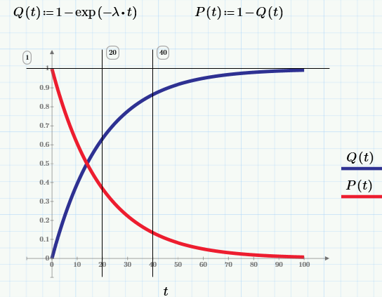
Differentiating Q (t), we obtain the expression for the probability density of the exponential distribution:
 ,
,
and from it the failure rate function: λ (t) = p (t) / P (t) = const = λ.
What did we get? That for an exponential distribution the failure rate is a constant value, and it coincides with the distribution parameter. This parameter is the main indicator of fault tolerance and is often called the λ-characteristic.
Moreover, if we now calculate the average time to the first failure - the same parameter MTTF (Mean Time To Failure), then we get that it is equal to MTTF = 1 / λ.

These are all remarkable properties of the exponential distribution. Why did we choose it as a description of failures? Because this is the simplest model - the model of the Poisson flow of events, which we have already considered in the article about the analysis of site conversion . Therefore, in the theory of reliability, the exponential distribution is most often used, for which, as we found out:
But this is not all, because for the exponential distribution it is especially easy to do the calculation of systems consisting of many elements. But about this - in the next article (to be continued).
Recently, I have quite a lot to work with calculations of reliability and risks, and in this article I will try to fill this gap, starting from my previous material (from the machine learning cycle) about the Poisson random process and supporting the text with calculations in Mathcad Express , which I repeat You can download this editor (read more about it here, please note that we need the latest version 3.1, as well as for the machine learning cycle). Matkadov's calculations themselves are here (along with the XPS copy).
1. Theory: basic fault tolerance characteristics
It seems that from the definition itself (Mean Time To Failure) its meaning is clear: how much (of course, on average, because the probabilistic approach) will serve the product. But in practice, this parameter is not very useful. Indeed, the information that the average time to hard disk failure is half a million hours can be a dead end. Much more informative is another parameter: the probability of breakdown or the probability of failure-free operation (FBG) for a certain period (for example, a year).
In order to understand how these parameters are related, and how, knowing MTTF, to calculate the FBG and the probability of failure, let us recall some information from mathematical statistics.
')
The key concept of the theory of reliability is the concept of failure, measured, respectively, by the interval indicator
Q (t) = probability that the product will fail by the time t.
Appropriately, the probability of failure-free operation (FBG, in the English terminology "reliability"):
P (t) = the probability that the product will work without abandoning the time t 0 = 0 until time t.
By definition, at time t 0 = 0, the product is in a healthy state, i.e. Q (0) = 0, and P (0) = 1.
Both parameters are interval characteristics of fault tolerance, since we are talking about the probability of failure (or vice versa, trouble-free operation) on the interval (0, t). If a failure is treated as a random event, then, obviously, Q (t) is, by definition, its distribution function. A point characteristic can be defined as
p (t) = dQ (t) / dt = probability density, i.e. the value of p (t) dt is equal to the probability that the failure will occur in a small neighborhood of dt of time t.
And finally, the most important (from a practical point of view) characteristic: λ (t) = p (t) / P (t) = failure rate.
This (attention!) Conditional probability density, i.e. probability density of failure at time t, provided that up to this considered time t the product has worked flawlessly.
The parameter λ (t) can be measured experimentally by testing a batch of products. If by the time t the operability has retained N items, then the estimate of λ (t) can be taken as the percentage of failures per unit time occurring in the neighborhood of t. More precisely, if in the period from t to t + dt n products fail, then the failure rate will be approximately equal to
λ (t) = n / (N * dt).
It is this λ-characteristic (in neglect of its dependence on time) that is most often cited in the passport data of various electronic components and various products. Only the question immediately arises: how to calculate the probability of failure-free operation and what is the average time to failure (MTTF).
But with it.
2. Exponential distribution
In the terminology we have just used, so far there have been no assumptions about the properties of a random variable — the point in time at which a product fails. Let us now specify the distribution function of the failure value by choosing as its exponential function with a single parameter λ = const (the meaning of which will be clear in a few sentences).
Differentiating Q (t), we obtain the expression for the probability density of the exponential distribution:
,and from it the failure rate function: λ (t) = p (t) / P (t) = const = λ.
What did we get? That for an exponential distribution the failure rate is a constant value, and it coincides with the distribution parameter. This parameter is the main indicator of fault tolerance and is often called the λ-characteristic.
Moreover, if we now calculate the average time to the first failure - the same parameter MTTF (Mean Time To Failure), then we get that it is equal to MTTF = 1 / λ.
These are all remarkable properties of the exponential distribution. Why did we choose it as a description of failures? Because this is the simplest model - the model of the Poisson flow of events, which we have already considered in the article about the analysis of site conversion . Therefore, in the theory of reliability, the exponential distribution is most often used, for which, as we found out:
- reliability of elements can be estimated by one number, since λ = const;
- using the well-known λ, it is quite simple to estimate the remaining reliability indices (for example, FBG for any time t)
- λ has good visibility
- λ is easy to measure experimentally
But this is not all, because for the exponential distribution it is especially easy to do the calculation of systems consisting of many elements. But about this - in the next article (to be continued).
Source: https://habr.com/ru/post/254893/
All Articles