Building analytical expressions ... for any objects - from the Pythagorean theorem to the pink panther and Sir Isaac Newton in Wolfram Language (Mathematica)

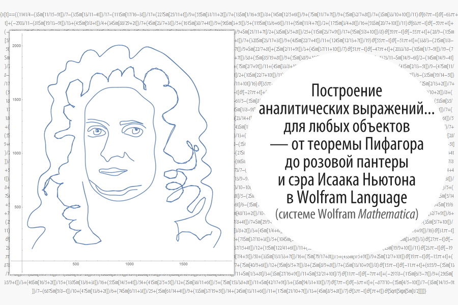
Translation of Michael Trott's post “ Making Formulas ... for Everything — From Pi to the Pink Panther to Sir Isaac Newton ."
Thanks for the help in translating Sylvia Torosyan .
Download the translation in the form of a Mathematica document that contains all the code used in the article here (archive, ~ 7 MB).

At Wolfram Research and Wolfram | Alpha, we love math and computation. Our favorite topics are algorithms that follow formulas and equations. For example, Mathematica can calculate millions of integrals (more precisely, an infinite number found in practice), and also Wolfram | Alpha knows hundreds of thousands of mathematical formulas (from Euler’s formula and BBP formulas for Pi to complex defined integrals containing sin (x) ) and a plurality of formulas physics (e.g., from Poiseuille's law to classical mechanics solutions spot particles in a rectangle or inverse distance capacity in four-dimensional space, in hyperspherical coordinates ), as well as less well-known formulas, such as formula d I rate wet dog shaking , the maximum height of the sand castle , or the time of cooking a turkey .

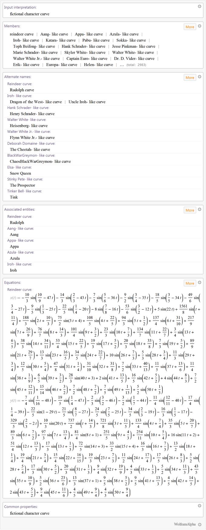
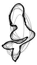
We recently added formulas for a variety of different shapes and objects. The Wolfram Blog | Alpha showed some examples of the formation of figures that were asked using mathematical equations and inequalities. Among the curves constructed are curves of images of fictional characters :


')


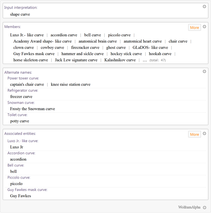
Curves outlines of objects :





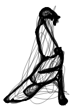
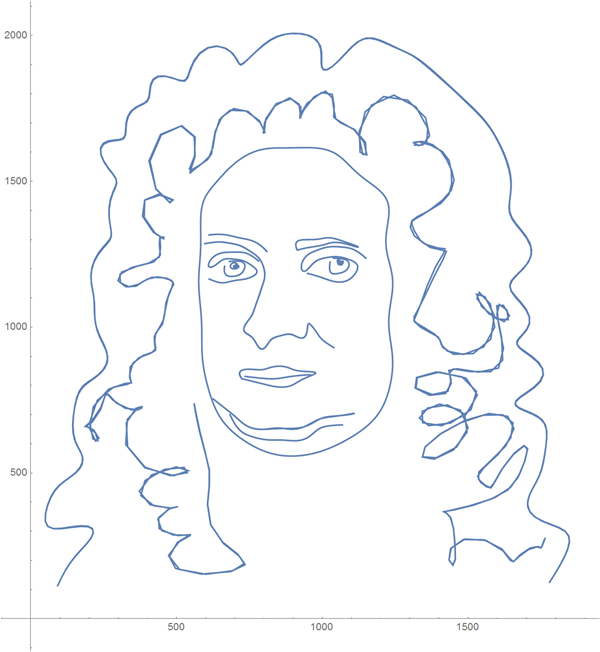
and, the most popular among our users, the curves of the images of real people :





Since these curves, in the mathematical sense, are similar to a lemniscate or a sheet of Descartes , they are more interesting from the point of view of their graphic representation than by their mathematical properties.

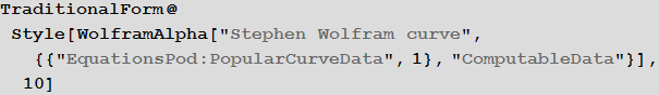
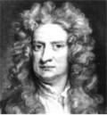
After Richard’s blog post was published, my colleague asked me, “How do you make an equation describing Stephen Wolfram’s face?” After a moment thinking about this question, I realized that it’s really amazing that the question is not that there is an analytical expression: a digital image (suppose for simplicity that it is black and white) is a rectangular array of gray values. Using this array, one can construct an interpolating function, even a polynomial. But such an explicit function would be very huge, hundreds of pages long, and would not be suitable for any practical application. In fact, the difficulty is how to obtain an analytical expression that would resemble a person’s face, so that it fits on one page and has a simple structure. An analytical expression for a curve that depicts Stephen Wolfram's face, approximately one page long, which is comparable to the size of a complex physics formula, such as, say, the cube's gravitational potential .





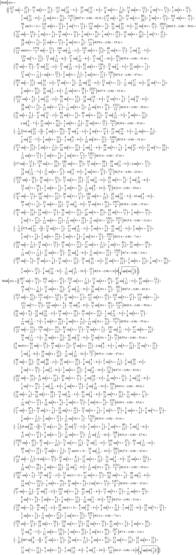
In this article I want to show how to generate this kind of equation. It is not at all surprising that in the article that tells “how to perform calculations ...” you will see a significant amount of Mathematica code, but I will start with simple introductory explanations.

Suppose you draw pencil lines on a piece of paper and assume that you draw only lines; no shading and no filling do not. Then the drawing will be made from a number of segments of the curve. A mathematical concept such as Fourier series allows us to write a finite mathematical formula for each of these line segments, which will describe them as you like.

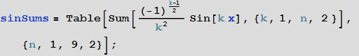
As a simple example, consider a series of functions. ,



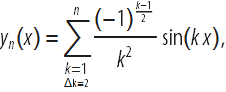
which are the sum of sinusoids of various frequencies and amplitudes. Here are the first few members of this function chain:







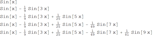
The graphical construction of this sequence of functions shows that with increasing n, the function tends to triangular function.





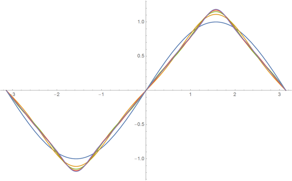
The sine function is an odd function, and as a result, any sums of functions of the form sin ( kx ) are also odd functions. If we use the cosine function, we’ll get even functions instead. The composition of the sine and cosine values ​​allows us to approximate more general curve shapes.

Summarizing the above, we replace the multiply in the series under consideration by and also we will set two rows, from sines and cosines, respectively:



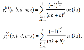
These functions allow you to approximate a wider class of functions:





It can be shown that any smooth curve y ( x ) can be arbitrarily well approximated on any interval using the Fourier series. Moreover, for smooth curves, the values ​​of the coefficients sin (kx) and cos (kx) tend to zero for large values ​​of k .

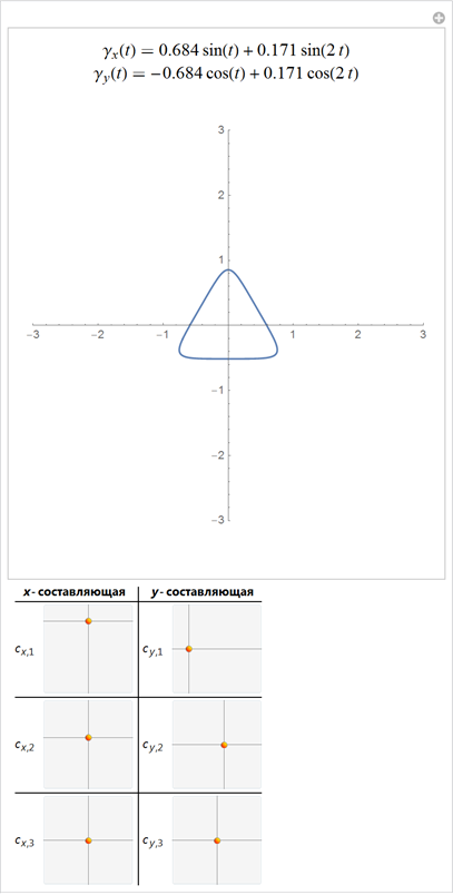
Now, considering a parametric curve , we can use this kind of superposition of sine and cosine functions independent for horizontal and vertical components.

The use of the sum of three sines and three cosines in each of the components already covers a wide variety of shapes, including circles and ellipses:



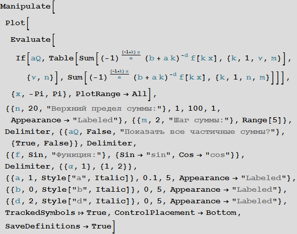
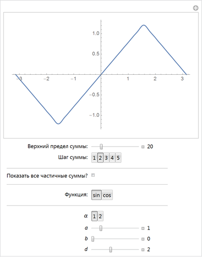
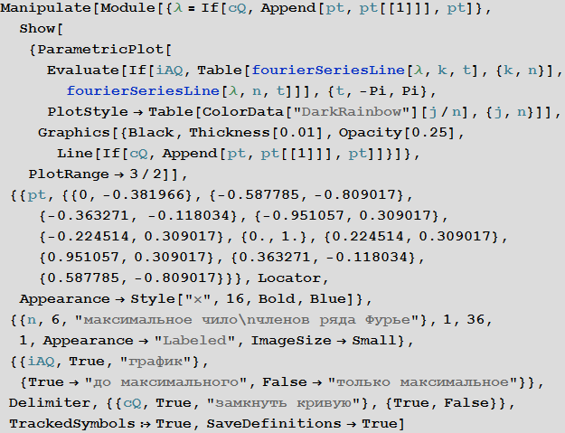
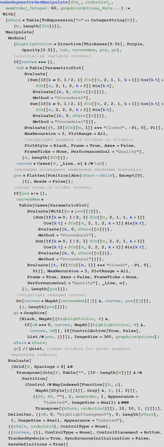
The following interactive demonstration allows us to explore the space of possible forms. 2D sliders change the corresponding coefficients before the functions of cosine and sine:





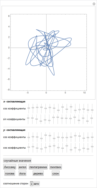
If we terminate the Fourier series expansion of a curve, say on the first n terms of the series, we get 4 n free parameters. In the space of all possible curves, most of the curves will look uninteresting, but for some values ​​of the coefficients, expansions will look like shapes in which you can see familiar shapes. However, even small changes in the coefficients of decomposition greatly change the shape. The following interactive example allows changing the initial 4 × 16 = 64 coefficients of a Fourier series of a curve. Using special sets of coefficients of Fourier series, we can get various recognizable figures.





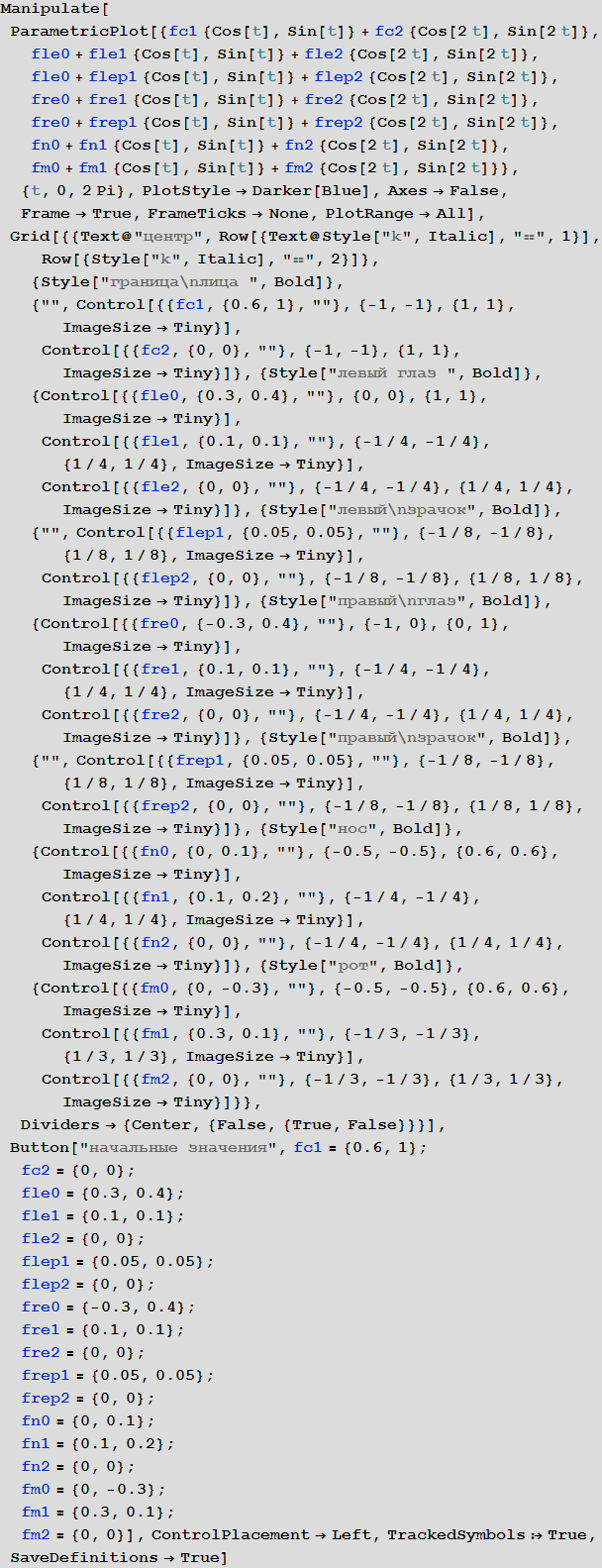
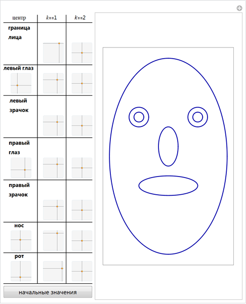
If we now take more than one curve, we will have all the necessary components to build a face-like image. The following interactive demonstration uses two eyes, two pupils, a nose and a mouth.





Now we will do the opposite: arrange a row of points (blue crosses) so that a line is formed that can be changed and build a curve that will approximate the given curve in Fourier series:









Note: Fourier series are not the only way to define approximating curves. We could use wavelets or splines , or encode curves piecewise through circular segments . Or with sufficient patience, with the help of the universality of the Riemann zeta function , we could find any figure inside the critical strip . (Surprisingly, any possible (fairly smooth) image, such as Jesus on toast, exists for some values ​​of the Riemann's zeta function ( s ) in the 0≤Re (s) ≤1 band, but we have no constructive way to find him.)

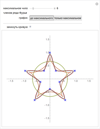
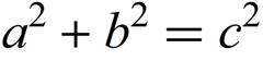
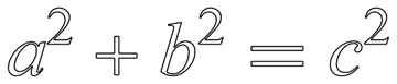
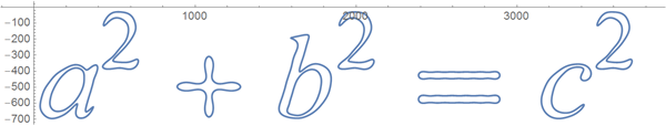
To demonstrate how to find simple formulas based on the Fourier series that approximate these figures, we start with an example: a figure with precise, clearly defined boundaries is a short formula. More specifically, we will use the well-known formula: the Pythagorean theorem.





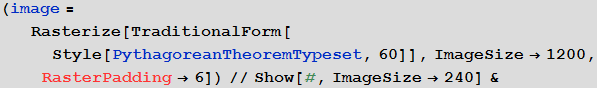
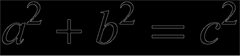
Rasterizing the equation will give the original image, which we will use:





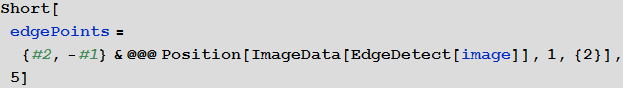
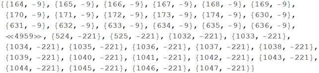
It is easy to get a set of all points describing the edges of characters using the EdgeDetect function.









Now that we have points that define edges, we can connect them with straight (or curvilinear) segments. The following pointListToLines function performs this operation. We start from a randomly selected point and find all the nearest points to it (using the fast Nearest function). We will continue this process until we find points of all fairly close points. Also make sure that there are no 180 degrees turns. To observe how curves are formed, we use the Monitor function.



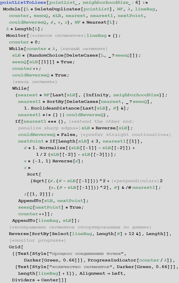
For the image of the recording of the Pythagorean theorem, we obtain 11 specific curves from boundary points.





Combining the sets of points and coloring the obtained curves, we will see the quite expected set of curves: the outer boundaries of the letters, the inner boundaries of the letters a and b , three squares, plus an equal sign.





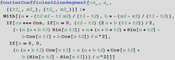
Now for each segment of the curve we need to find the Fourier series (x and y components), which approximates the segment. Guided by the usual definition of the Fourier series of the function f (x), we know that the coefficients of the series are integrals of the function f (x) multiplied by cos (kx) and sin (kx). But while we have a lot of points, not functions. To convert them into functions that we can integrate, create B- splines of the curve for each of its segments. The parametrized variable B -spline of the curve will be the variable of integration. (Using B- splines instead of piecewise linear interpolation between points will give us additional advantages in approximating strongly broken curves.)





We can find the integrals needed to obtain the Fourier coefficients using numerical integration, however, a faster way is to use the Fast Fourier Transform ( FFT ) to obtain the Fourier coefficients.

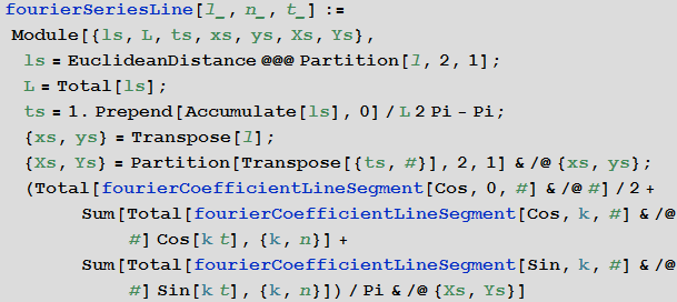
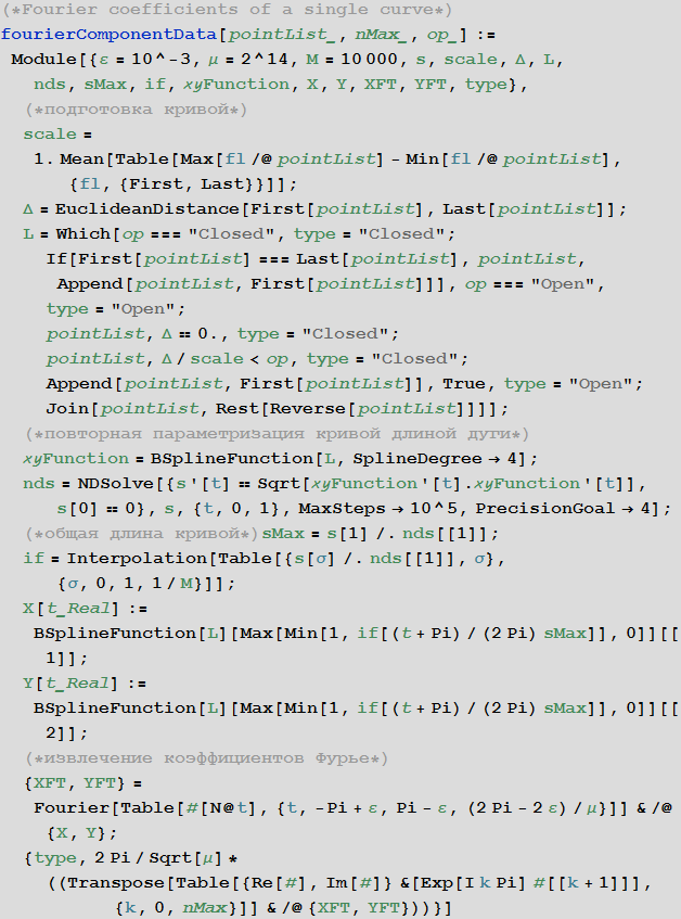
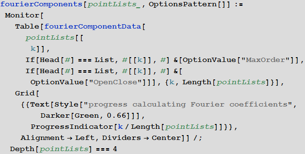
To obtain more uniform curves, we will take another step: re-parameterize the interpolated spline curve, consisting of a set of curve segments, with the help of a new parameter - the arc length. The fourierComponents function implements the creation of a B-spline curve , re-parameterization by arc length and calculates FTT to get the Fourier coefficients. We also consider whether a segment of a curve is open or closed to avoid the Gibbs phenomenon . (The above demonstration of the approximation of a pentagram clearly shows the Gibbs phenomenon in case the “close curve” box is unchecked.)









For continuous function, we expect the average value of the rate of decrease for the kth coefficient of the Fourier series. This effect should also be retained for the coefficients of the Fourier series calculated by us. This means that on average, the 10th Fourier coefficient accounts for only 1% of the absolute value compared with the first. This makes it possible to trim the Fourier series in not very high orders, since we do not want to get formulas that are too large. The expression below calculates the average exponent of the rate of decrease of the Fourier components for the above curve. . (The value is slightly less than 2 due to the discretization of points in the B-spline curves.)





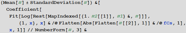
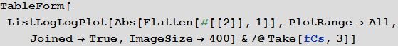
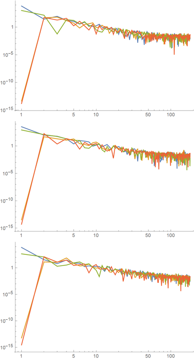
Below is a graph on a logarithmic scale along both axes with the absolute values ​​of the coefficients of the Fourier series for the first three curves. However, the general trend with respect to, say, quadratic attenuation for Fourier coefficients shows that the magnitude of neighboring coefficients often fluctuates more than the average value of the loss of the coefficients as a whole.





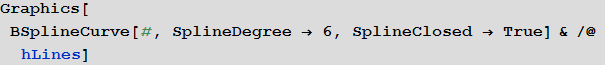
Multiplying the Fourier coefficients by cos (kt) and sin (kt) and summing these expressions gives us the desired parametrization of the curves.



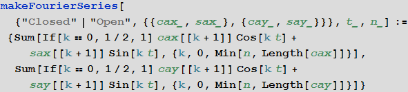
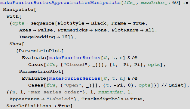
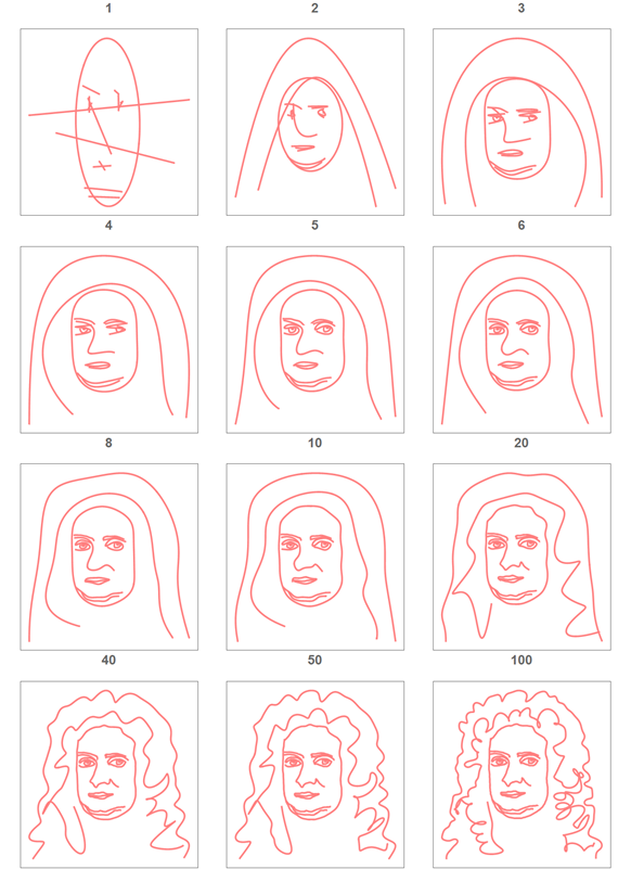
The makeFourierSeriesApproximationManipulate function visualizes curve approximations depending on how many row members are taken.



For the picture corresponding to the Pythagorean theorem, starting with a dozen ellipses, we quickly form the original image, increasing the number of members of the Fourier series.





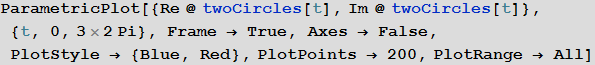
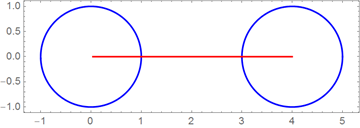
We want to define an analytical expression for the whole equation, even if this expression consists of non-intersecting segments of a curve. To achieve this, we use the periodicity of the members of the Fourier series, having a period of 2 π , in order to depict each of the segments on the corresponding segment: [0,2π], [4 π, 6 π], [8 π, 10 π], ..., and in the intervals (2π, 4π), (6 π, 8 π), ..., we will have purely imaginary coordinates of the curve. On these segments, the curve cannot be depicted, which means that we get a set of non-intersecting segments of the curve. Below this construction is shown for a set of two circles:







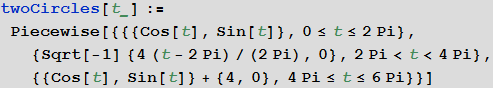
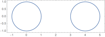
The graph below shows separately the real and imaginary parts of the complex-valued parametrization constructed above. The red line shows the purely imaginary parameter values ​​from the interval [2π, 4π].





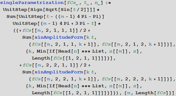
Since we want the final formula for the curves to look as short and simple as possible, we replace the sum in the formula a cos (kt) + b sin (kt) with A sin (k t + φ) using the sinAmplitudeForm function, as well as rounds the approximate coefficients of the Fourier series to the nearest rational numbers. Instead of Piecewise , we use the UnitStep function in the final formula to separate different segments of the curve from each other. We enumerate the real segments explicitly, and all the segments that should not be drawn are given by the expression .







Now we have everything to write the final parametrization {x (t), y (t)} of the picture, which shows the equality that defines the Pythagorean theorem:











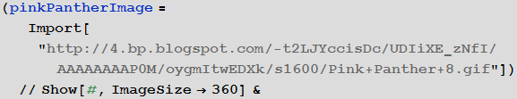
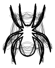
After we have discussed the basic ideas of parametrization, let's look at a funnier example, say Pink Panther . Looking through the image search results by the Bing search engine, we quickly find an image that is suitable for parameterization in the form of a " closed form ."

Let's use the following image:





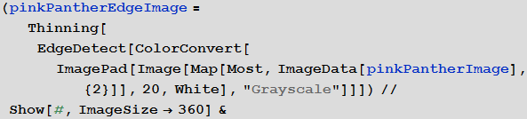
Use the EdgeDetect function to find all the borders of a panther’s face.







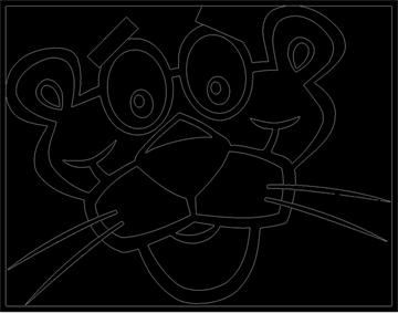
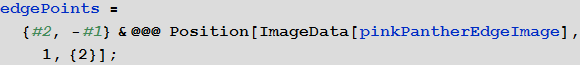
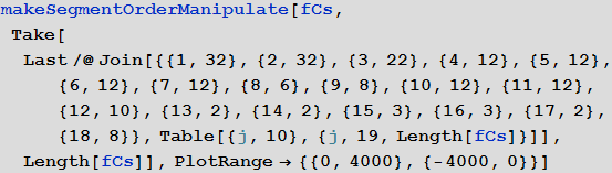
Connecting the edges of the curve, we get about 20 segments. (By changing the additional second and third argument of the pointListToLines function, we get fewer or more segments.)





. , ; pointListToLines . .





, , .



, , 20 , , .











, , .





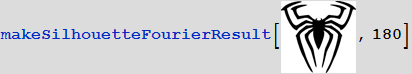
. makeSilhouetteFourierResult . : 1) ; 2) , . .



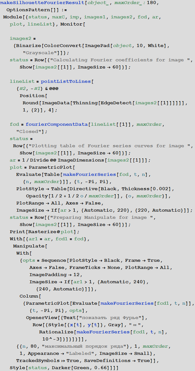
. 4 : ; -; , .

























. . , . , , . ( . .) , :





, , , .







, .





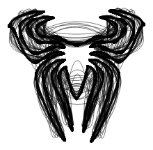
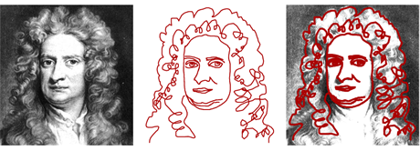
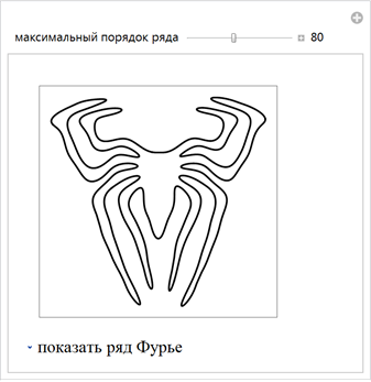
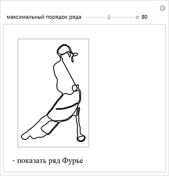
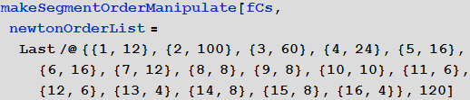
, 16 . .



, :





. , , . , .





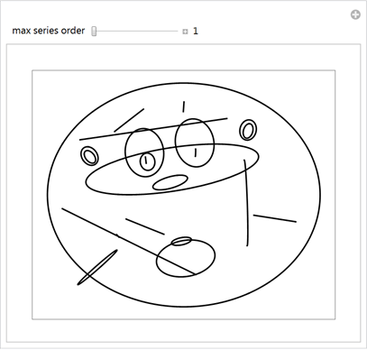
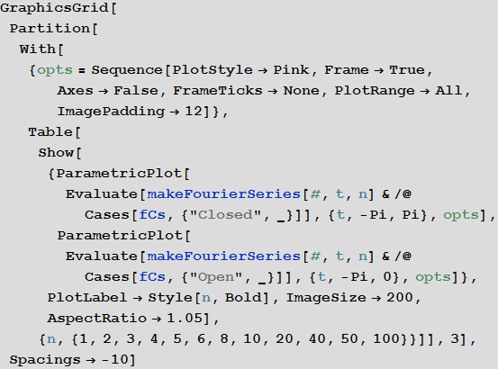
50 :





, , :







:





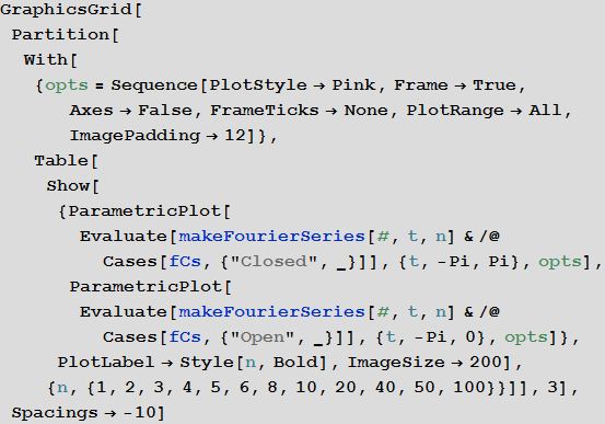
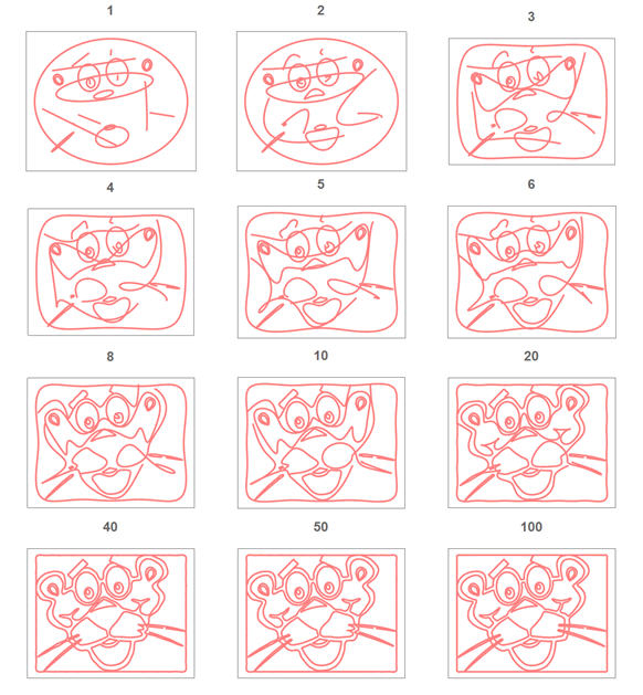
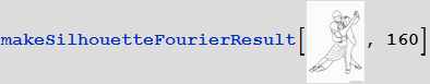
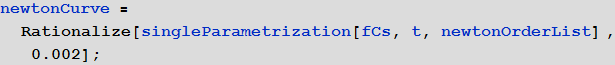
This concludes today's discussion on how to construct curves that resemble the faces of people, fictional characters, animals, or other forms. Next time we will discuss the infinite graphical possibilities that arise from the above formulas and how you can use this kind of equation for a variety of images.