Genetic algorithm - visual implementation
About four years ago, in the university I heard about such an optimization method as a genetic algorithm. He was reported exactly two facts everywhere: he is cool and he does not work. Rather, it works, but slowly, unreliably, and nowhere should it be used. But he can beautifully demonstrate the mechanisms of evolution. In this article, I will show a beautiful way to see the evolutionary processes in person, using the example of this simple method. You just need a little math, programming, and all this spice up the imagination.
So what is a genetic algorithm? First of all, this is a multi-dimensional optimization method, i.e. method of finding the minimum of a multidimensional function. Potentially, this method can be used for global optimization, but with this there are difficulties, I will describe them later.
The very essence of the method lies in the fact that we modulate the evolutionary process: we have some kind of population (set of vectors) that multiplies, which is affected by mutations and natural selection is made based on minimizing the objective function. Let us consider these processes in more detail.
So, first of all, our population should multiply . The basic principle of reproduction is that a descendant resembles its parents. Those. we have to specify some sort of inheritance mechanism. And it would be better if it includes an element of chance. But the speed of development of such systems is very low - the diversity of genetic drops, the population degenerates. Those. the value of the function stops being minimized.
')
To solve this problem, a mutation mechanism was introduced, which consists in the random change of some individuals. This mechanism allows you to bring something new to genetic diversity.
The next important mechanism is selection . As has been said, selection is the selection of individuals (it is possible from only born, and it is possible from all - practice shows that this does not play a decisive role), which better minimize the function. Usually, as many individuals are selected as before reproduction so that from epoch to epoch we have a constant number of individuals in the population. It is also customary to select "lucky ones" - a certain number of individuals, which, perhaps, poorly minimize the function, but will introduce diversity in future generations.
These three mechanisms are often insufficient to minimize the function. So the population degenerates - sooner or later the local minimum clogs the entire population with its value. When this happens, they carry out a process called shake - up (in nature, analogies are global cataclysms), when almost the entire population is destroyed, and new (random) individuals are added.
Here is a description of the classical genetic algorithm, it is simple to implement and there is a place for imagination and research.
So, when I decided that I wanted to try to implement this legendary (albeit unlucky) algorithm, we were talking about what would I be minimizing? Usually they take some terrible multidimensional function with sines, cosines, etc. But this is not very interesting and generally not obvious. An unpretentious idea came - an image is perfectly suitable for displaying a multidimensional vector, where the value is responsible for brightness. Thus, we can introduce a simple function - the distance to our target image, measured in the difference in brightness of pixels. For simplicity and speed, I took images with a brightness of 0, or 255.
From the point of view of mathematics, such optimization is a mere trifle. The graph of such a function is a huge multidimensional "pit" (like a three-dimensional parabaloid in the figure), which you inevitably roll into if you follow the gradient. The only local minimum is global.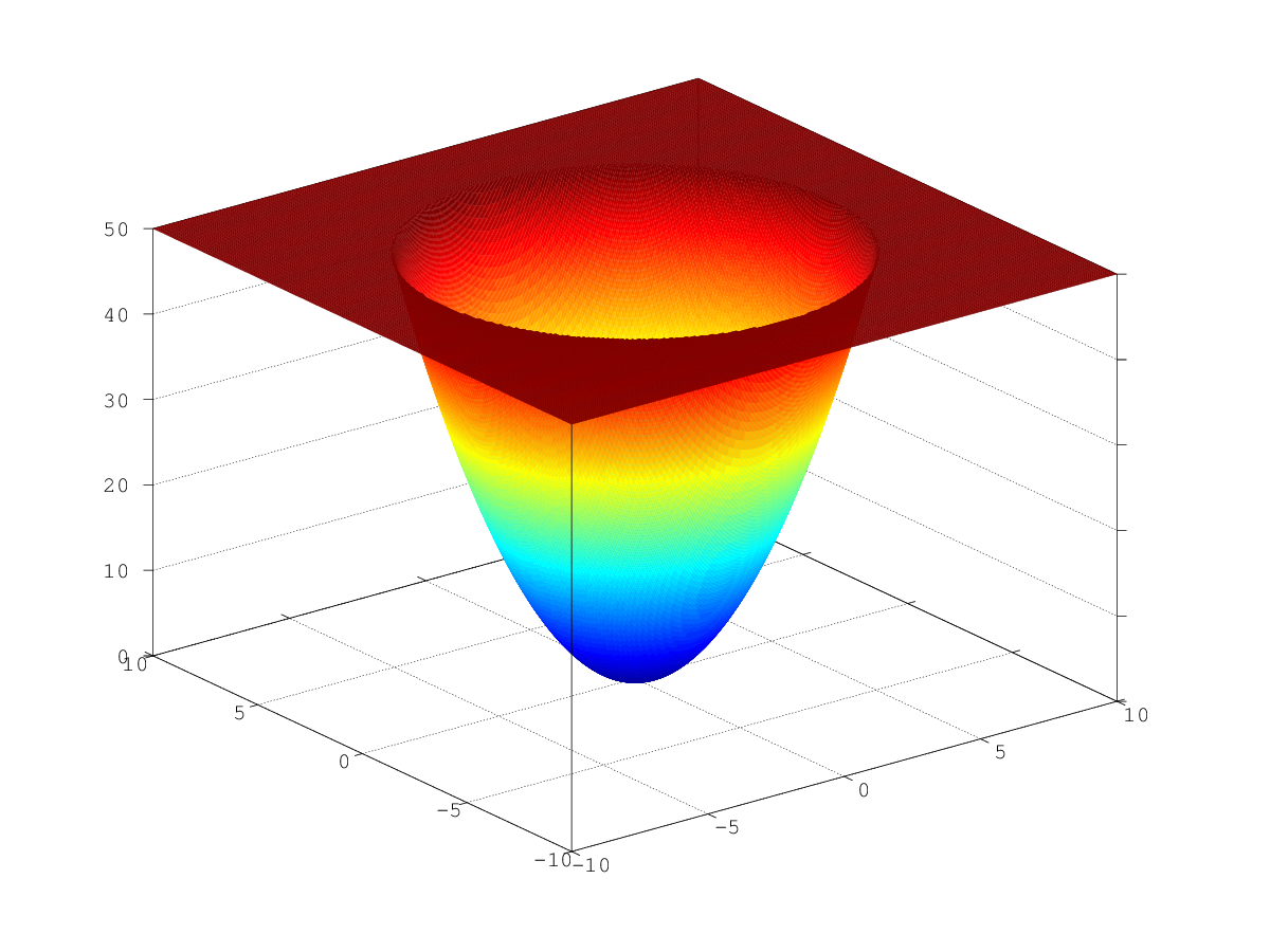 .
.
The only problem is that already close to the minimum, the number of paths through which you can go down is greatly reduced, and we have as many directions as dimensions (i.e., the number of pixels). Obviously, this task should not be solved with the help of a genetic algorithm, but we can look at interesting processes occurring in our population.
All the mechanisms described in the first paragraph were implemented. Reproduction was carried out by simply crossing random pixels from the "mother" and the "father". Mutations were made by changing the value of a random pixel in a random individual to the opposite. And the shaking was made, if the minimum does not change over five steps. Then an “extreme mutation” is made - the replacement is more intense than usual.
I used nonograms (“Japanese scanwords”) as original pictures, but, in truth, you can just take black squares - there is absolutely no difference. Below are the results for multiple images. Here, for all but the “house”, the number of mutations was 100 on average for each individual, there were 100 individuals in the population, and during reproduction the population increased 4 times. The lucky ones were 30% in each era. For the house values were chosen smaller (30 individuals in the population, mutations of 50 per individual).
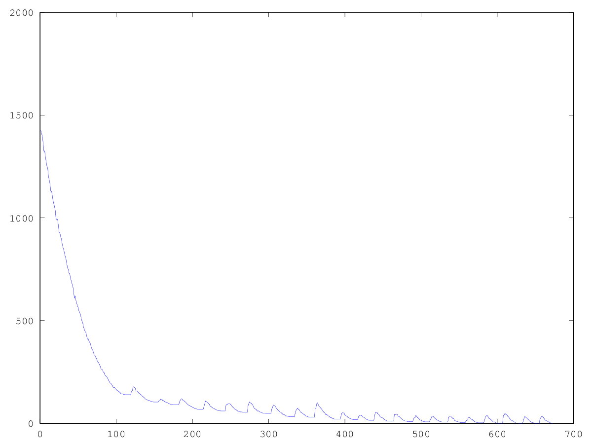
Experimentally, I found that using the “lucky ones” in breeding lowers the rate of aspiration of the population to a minimum, but it helps to get out of stagnation — without the “lucky ones,” the stagnation will be constant. What can be seen from the graphs: the left graph is the development of the “Pharaoh” population with the lucky ones, the right one - without the lucky ones.

Thus, we see that this algorithm allows us to solve the problem posed, albeit for a very long time. Too many shakes, in the case of large images, can solve a larger number of individuals in the population. I leave the optimal selection of parameters for different dimensions beyond the scope of this post.
As it was said, local optimization is a rather trivial task, even for multidimensional cases. It is much more interesting to see how the algorithm will cope with global optimization. But for this you first need to build a function with a set of local minima. And this is not so difficult in our case. It is enough to take a minimum from the distance to several images (house, dinosaur, fish, boat). Then the original algorithm will "roll" into some random hole. And you can just run it several times.
But there is a more interesting solution to this problem: you can understand that we have slipped into a local minimum, make a strong shake-up (or even initiate individuals altogether), and further add penalties when approaching a known minimum. As you can see, the pictures alternate. I note that we have no right to touch the original function. But we can memorize local minima and add fines on our own.
This picture shows the result when, when a local minimum is reached (severe stagnation), the population simply dies out.
Here the population dies out, and a small fine is added (at the rate of the usual distance to a known minimum). This greatly reduces the likelihood of repetitions.
It is more interesting when the population does not die out, but simply begins to line up under the new conditions (the next figure). This is achieved with a fine of 0.000001 * sum ^ 4. In this case, new images become a bit noisy:
This noise is eliminated by limiting the penalty to max (0.000001 * sum ^ 4, 20). But we see that the fourth local minimum (dinosaur) cannot be reached - most likely because it is too close to some other.
What conclusions can we draw from modeling, I’m not afraid of this word? First of all, we see sexual reproduction is the most important engine of development and adaptability. But it is not enough. The role of random, small changes is extremely important. They provide the emergence of new species of animals in the process of evolution, and in our country it provides a diversity of the population.
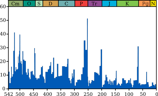
The most important role in the evolution of the Earth was played by natural disasters and mass extinctions (the extinction of dinosaurs, insects, etc. - there were about ten large ones - see the diagram below). This was confirmed by our modeling. And the selection of "lucky ones" showed that the weakest organisms today can in the future be the basis for future generations.
As they say, everything is as in life. This “make yourself evolution” method clearly shows interesting mechanisms and their role in development. Of course, there are many more worthwhile evolutionary models (based, of course, on diffures), which take into account more factors that are more close to life. Of course, there are more efficient optimization methods.
I wrote a program on Matlab (or rather, even on Octave), because everything here is a dummy matrix, and there are tools for working with pictures. The source code is attached.
Briefly about the algorithm
So what is a genetic algorithm? First of all, this is a multi-dimensional optimization method, i.e. method of finding the minimum of a multidimensional function. Potentially, this method can be used for global optimization, but with this there are difficulties, I will describe them later.
The very essence of the method lies in the fact that we modulate the evolutionary process: we have some kind of population (set of vectors) that multiplies, which is affected by mutations and natural selection is made based on minimizing the objective function. Let us consider these processes in more detail.
So, first of all, our population should multiply . The basic principle of reproduction is that a descendant resembles its parents. Those. we have to specify some sort of inheritance mechanism. And it would be better if it includes an element of chance. But the speed of development of such systems is very low - the diversity of genetic drops, the population degenerates. Those. the value of the function stops being minimized.
')
To solve this problem, a mutation mechanism was introduced, which consists in the random change of some individuals. This mechanism allows you to bring something new to genetic diversity.
The next important mechanism is selection . As has been said, selection is the selection of individuals (it is possible from only born, and it is possible from all - practice shows that this does not play a decisive role), which better minimize the function. Usually, as many individuals are selected as before reproduction so that from epoch to epoch we have a constant number of individuals in the population. It is also customary to select "lucky ones" - a certain number of individuals, which, perhaps, poorly minimize the function, but will introduce diversity in future generations.
These three mechanisms are often insufficient to minimize the function. So the population degenerates - sooner or later the local minimum clogs the entire population with its value. When this happens, they carry out a process called shake - up (in nature, analogies are global cataclysms), when almost the entire population is destroyed, and new (random) individuals are added.
Here is a description of the classical genetic algorithm, it is simple to implement and there is a place for imagination and research.
Formulation of the problem
So, when I decided that I wanted to try to implement this legendary (albeit unlucky) algorithm, we were talking about what would I be minimizing? Usually they take some terrible multidimensional function with sines, cosines, etc. But this is not very interesting and generally not obvious. An unpretentious idea came - an image is perfectly suitable for displaying a multidimensional vector, where the value is responsible for brightness. Thus, we can introduce a simple function - the distance to our target image, measured in the difference in brightness of pixels. For simplicity and speed, I took images with a brightness of 0, or 255.
From the point of view of mathematics, such optimization is a mere trifle. The graph of such a function is a huge multidimensional "pit" (like a three-dimensional parabaloid in the figure), which you inevitably roll into if you follow the gradient. The only local minimum is global.
.The only problem is that already close to the minimum, the number of paths through which you can go down is greatly reduced, and we have as many directions as dimensions (i.e., the number of pixels). Obviously, this task should not be solved with the help of a genetic algorithm, but we can look at interesting processes occurring in our population.
Implementation
All the mechanisms described in the first paragraph were implemented. Reproduction was carried out by simply crossing random pixels from the "mother" and the "father". Mutations were made by changing the value of a random pixel in a random individual to the opposite. And the shaking was made, if the minimum does not change over five steps. Then an “extreme mutation” is made - the replacement is more intense than usual.
I used nonograms (“Japanese scanwords”) as original pictures, but, in truth, you can just take black squares - there is absolutely no difference. Below are the results for multiple images. Here, for all but the “house”, the number of mutations was 100 on average for each individual, there were 100 individuals in the population, and during reproduction the population increased 4 times. The lucky ones were 30% in each era. For the house values were chosen smaller (30 individuals in the population, mutations of 50 per individual).
Experimentally, I found that using the “lucky ones” in breeding lowers the rate of aspiration of the population to a minimum, but it helps to get out of stagnation — without the “lucky ones,” the stagnation will be constant. What can be seen from the graphs: the left graph is the development of the “Pharaoh” population with the lucky ones, the right one - without the lucky ones.
Thus, we see that this algorithm allows us to solve the problem posed, albeit for a very long time. Too many shakes, in the case of large images, can solve a larger number of individuals in the population. I leave the optimal selection of parameters for different dimensions beyond the scope of this post.
Global optimization
As it was said, local optimization is a rather trivial task, even for multidimensional cases. It is much more interesting to see how the algorithm will cope with global optimization. But for this you first need to build a function with a set of local minima. And this is not so difficult in our case. It is enough to take a minimum from the distance to several images (house, dinosaur, fish, boat). Then the original algorithm will "roll" into some random hole. And you can just run it several times.
But there is a more interesting solution to this problem: you can understand that we have slipped into a local minimum, make a strong shake-up (or even initiate individuals altogether), and further add penalties when approaching a known minimum. As you can see, the pictures alternate. I note that we have no right to touch the original function. But we can memorize local minima and add fines on our own.
This picture shows the result when, when a local minimum is reached (severe stagnation), the population simply dies out.
Here the population dies out, and a small fine is added (at the rate of the usual distance to a known minimum). This greatly reduces the likelihood of repetitions.
It is more interesting when the population does not die out, but simply begins to line up under the new conditions (the next figure). This is achieved with a fine of 0.000001 * sum ^ 4. In this case, new images become a bit noisy:
This noise is eliminated by limiting the penalty to max (0.000001 * sum ^ 4, 20). But we see that the fourth local minimum (dinosaur) cannot be reached - most likely because it is too close to some other.
Biological interpretation
What conclusions can we draw from modeling, I’m not afraid of this word? First of all, we see sexual reproduction is the most important engine of development and adaptability. But it is not enough. The role of random, small changes is extremely important. They provide the emergence of new species of animals in the process of evolution, and in our country it provides a diversity of the population.
The most important role in the evolution of the Earth was played by natural disasters and mass extinctions (the extinction of dinosaurs, insects, etc. - there were about ten large ones - see the diagram below). This was confirmed by our modeling. And the selection of "lucky ones" showed that the weakest organisms today can in the future be the basis for future generations.
As they say, everything is as in life. This “make yourself evolution” method clearly shows interesting mechanisms and their role in development. Of course, there are many more worthwhile evolutionary models (based, of course, on diffures), which take into account more factors that are more close to life. Of course, there are more efficient optimization methods.
PS
I wrote a program on Matlab (or rather, even on Octave), because everything here is a dummy matrix, and there are tools for working with pictures. The source code is attached.
Source
function res = genetic(file) %generating global AB; im2line(file); dim = length(A(1,:)); count = 100; reprod = 4; mut = 100; select = 0.7; stagn = 0.8; pop = round(rand(count,dim)); res = []; B = []; localmin = []; localcount = []; for k = 1:300 %reproduction for j = 1:count * reprod pop = [pop; crossingover(pop(floor(rand() * count) + 1,:),pop(floor(rand() * count) + 1,:))]; end %mutation idx = 10 * (length(res) > 5 && std(res(1:5)) == 0) + 1; for j = 1:count * mut a = floor(rand() * count) + 1; b = floor(rand() * dim) + 1; pop(a,b) = ~pop(a,b); end %selection val = func(pop); val(1:count) = val(1:count) * 10; npop = zeros(count,dim); [s,i] = sort(val); res = [s(1) res]; opt = pop(i(1),:); fn = sprintf('result/%05d-%d.png',k,s(1)); line2im(opt*255,fn); if (s(1) == 0 || localcount > 10) localmin = []; localcount = []; B = [B; opt]; % pop = round(rand(count,dim)); continue; % break; end for j = 1:floor(count * select) npop(j,:) = pop(i(j),:); end %adding luckers for j = (floor(count*select)+1) : count npop(j,:) = pop(floor(rand() * count) + 1,:); end %fixing stagnation if (length(res) > 5 && std(res(1:5)) == 0) if (localmin == res(1)) localcount = localcount+1; else localcount = 1; end localmin = res(1); for j = 1:count*stagn a = floor(rand() * count) + 1; npop(a,:) = crossingover(npop(a,:),rand(1,dim)); end end pop = npop; end res = res(length(res):-1:1); end function res = crossingover(a, b) x = round(rand(size(a))); res = a .* x + b .* (~x); end function res = func(v) global AB; res = inf; for i = 1:size(A,1) res = min(res,sum(v ~= A(i,:),2)); end for i = 1:size(B,1) res = res + max(0.000001 * sum(v == B(i,:),2) .^ 4,20); end end function [] = im2line(files) global A sz; A = []; files = cellstr(files); for i = 1:size(files,1) imorig = imread(char(files(i,:))); sz = size(imorig); A = [A; reshape(imorig,[1 size(imorig,1)*size(imorig,2)])]; end A = A / 255; end function [] = line2im(im,file) global sz; imwrite(reshape(im*255,sz),file); end Source: https://habr.com/ru/post/254759/
All Articles