Determine the weight of chess pieces by regression analysis

Hello, Habr!

This article focuses on a small programmer etude on machine learning. His idea came to me during the passage of the Machine Learning course, which is well-known to many here, read by Andrew Ng on Curser. After becoming acquainted with the methods described in the lectures, I wanted to apply them to some real problem. It did not take long to search for a topic - as the subject area, it simply suggested an optimization of one’s own chess engine.

Introduction: about chess programs

We will not go deep into the architecture of chess programs in detail - this could be the subject of a separate publication or even a series of them. Consider only the most basic principles. The main components of almost any non-protein chess player are the search and evaluation of positions .
')
The search is a search of options, that is, an iterative deepening of the game tree. The evaluation function displays a set of positional signs on a numerical scale and serves as a target function for finding the best move. It is applied to the leaves of a tree, and gradually “returns” to its original position (root) using the alpha-beta procedure or its variations.

Strictly speaking, this score can take only three values: win, lose or draw - 1, 0 or ½. By the Zermelo theorem, for any given position, it is uniquely determined. In practice, due to a combinatorial explosion, no computer is able to calculate the variants to the leaves of a complete game tree (an exhaustive analysis in endgame databases is a separate case; 32-figured tables will not appear in the foreseeable future ... and in the boundless, most likely, also). Therefore, the programs work in the so-called Shannon model — they use a truncated game tree and an approximate estimate based on various heuristics.

Search and evaluation do not exist independently of each other, they must be well balanced. Modern reboring algorithms are no longer a “blunt” search of options; they include numerous special rules, including those related to position evaluation.

The first such search enhancements appeared at the dawn of chess programming, in the 60s of the 20th century. We can mention, for example, the technique of the forced variant (PV) - the extension of individual branches of the search until the position “calms down” (the shahs and mutual taking of figures are completed). Extensions significantly increase the tactical vigilance of a computer, and also lead to the fact that the search tree becomes very heterogeneous - the length of individual branches can be several times longer than the length of neighboring, less prospective. Other improvements to the search, on the contrary, represent a cutoff or reduction of the search - and here the same static assessment can serve as a criterion for discarding bad options.

Parameterization and improvement of search by machine learning methods is a separate interesting topic, but now we will leave it aside. For now let's deal only with the evaluation function.

How the computer evaluates the position

A static score is a linear combination of various attributes of a position, taken with some weights. What are these signs? First of all, the number of pieces and pawns on both sides. The next important sign is the position of these figures, centralization, the occupation of long-range figures with open lines and diagonals. Experience shows that taking into account only these two factors - the sum of the material and the relative value of the fields (fixed in the form of tables for each type of figures) - if there is a quality search, it can already provide the strength of the game in the range up to 2000-2200 Elo points. This is the level of a good first grade or master candidate.

Further refinement of the assessment may include more and more subtle signs of the chess position: the presence and advancement of the passing pawns, the proximity of the pieces to the position of the enemy king, his pawn cover, etc. function of several dozen signs . All of them are described in detail in the book The Machine Plays Chess, the bibliographic reference to which is given at the end of the article.

One of the most "clever" evaluation functions was at the car Deep Blue, famous for its matches with Kasparov in 1996-97. (You can read a detailed history of these matches in a recent series of articles on Geektimes .)

It is widely believed that the power of Deep Blue was based solely on the tremendous speed of searching through the options. 200 million positions per second, complete (without cut-offs) enumeration by 12 half-moves - the chess programs on modern hardware are just approaching such parameters. However, it was not only speed. In terms of the "chess knowledge" in the evaluation function, this machine is also far superior to all. Deep Blue score was implemented in hardware and included up to 8,000 different signs. Strong grandmasters were attracted to adjust its coefficients (it is reliably known about working with Joel Benjamin, test batches with different versions of the machine were played by David Bronstein).

Without having such resources as creators of Deep Blue, we will limit the task. Of all the signs of the position that are taken into account for the calculation of the assessment, we take the most significant - the ratio of the material on the board.

The cost of figures: the simplest models

If you take any chess book for beginners, immediately after the chapter with a description of the chess moves is usually given a table of the comparative value of the figures, something like this:

Type of	Cost of
Pawn	one
Horse	3
Elephant	3
Rook	five
Queen	9
King	∞

The king is sometimes credited with the final cost, obviously greater than the sum of all the material on the board — for example, 200 units. In this study, we will leave His Majesty alone, and we will not consider kings at all. Why? The answer is simple: they are always present on the board, so their material values are mutually subtracted, and they do not affect the overall balance of power.

Given the value of the figures should be considered only as some basic benchmarks. In reality, the pieces may “become more expensive” and “cheaper” depending on the situation on the board, as well as on the stage of the game. As a first-order amendment, combinations of two or three figures — one’s own and one’s opponent’s are usually considered.

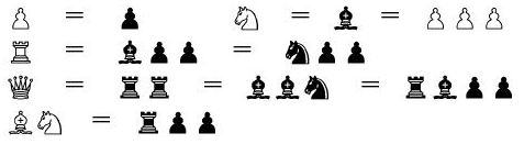
This is how the third world champion José Raul Capablanca evaluated various combinations of material in his classic “Chess Game Tutorial”:

From the point of view of the general theory, the elephant and the horse should be considered equally valuable, although, in my opinion, the elephant in most cases turns out to be a stronger figure. Meanwhile, it is considered quite established that two bishops are almost always stronger than two horses.

The bishop in the game against pawns is stronger than the knight, and together with the pawns it also turns out to be stronger against the rook than the knight. The bishop and the rook are also stronger than the knight and the rooks, but the queen and knight may turn out to be stronger than the queen and bishop. An elephant often costs more than three pawns, but this is rarely said about a horse; he may even be weaker than three pawns.

The rook is equal in strength to the knight and two pawns, or to the bishop and two pawns, but, as mentioned above, the bishop is stronger than the knight in the fight against the rook. Two rooks are somewhat stronger than the queen. They are slightly weaker than two horses and an elephant and even weaker than two elephants and a horse. The power of the horses decreases as the exchange of pieces on the board, the power of the rooks, on the contrary, increases.

Finally, as a rule, three light pieces are stronger than a queen.

It turns out that most of these rules can be satisfied by remaining within the linear model, and simply slightly shifting the value of the figures from their "school" values. For example, in one of the articles the following boundary conditions are given:

B > N > 3P B + N = R + 1.5P Q + P = 2R

And values satisfying them:

 P = 100 N = 320 B = 330 R = 500 Q = 900 K = 20000

The names of the variables correspond to the designations of pieces in the English notation: P - pawn, N - knight, B - bishop, R - rook, Q - queen, K - king. The costs hereinafter are indicated in hundredths of a pawn.

In fact, this set of values is not the only solution. Moreover, even non-compliance with some of the “inequalities to them. Capablanca will not lead to a sharp drop in the strength of the game of the program, but only affect its style features.

As an experiment, I spent a small match-tournament of four versions of my GreKo engine with different weights of figures against three other programs - each version played 3 matches for 200 games with ultra-small time control (1 second + 0.1 seconds per turn). The results are shown in the table:

Version	Pawn	Horse	Elephant	Rook	Queen	vs. Fruit 2.1	vs. Crafty 23.4	vs. Delfi 5.4	Rating
GreKo 12.5	100	400	400	600	1200	61.0	76.0	71.0	2567
Greko a	100	300	300	500	900	55.0	69.0	73.0	2552
Greko b	100	320	330	500	900	57.0	71.0	64.0	2548
Greko c	100	325	325	550	1100	72.5	74.5	69.0	2575

We see that some variations in the scales of the figures lead to fluctuations in the strength of the game in the range of 20-30 points of Elo. Moreover, one of the test versions showed an even better result than the main version of the program. However, it is premature to unequivocally assert that the game is being enhanced on such a small number of games - the confidence interval for calculating the rating is a comparable amount of several dozen Elo points.

The “classic” values of chess material were obtained intuitively, by the chess players understanding their practical experience. Attempts have also been made to bring some mathematical basis for these values - for example, on the basis of the mobility of figures, the number of fields that they can keep under control. We will try to approach the question experimentally - based on the analysis of a large number of chess games. To calculate the value of figures, we do not need an approximate assessment of the positions of these parties - only their results, as the most objective measure of success in chess.

Material overweight and logistic curve

For statistical analysis, a PGN file was taken, containing almost 3000 chess games in a blitz between 32 different chess engines, in the range from 1800 to 3000 Elo points. With the help of a specially written utility for each game, a list of material relationships arising on the board was compiled. Each correlation of the material did not fall into the statistics immediately after the capture of a piece or the transformation of a pawn - first, there should have been a reciprocal capture or several "quiet" moves. Thus, short-term “material jumps” were filtered by 1-2 turns during exchanges.

Then, using the scale “1-3-3-5-9” already known to us, the material balance of the position was calculated, and for each of its values (from -24 to 24), the number of points scored by White was accumulated. The statistics obtained are presented in the following graph:

On the x-axis, the material balance of the ΔM position from the point of view of White, in pawns. It is calculated as the difference between the total value of all white pieces and pawns and the same value for black. On the y axis, the sample is the expected result of the game (0 is Black’s victory, 0.5 is a draw, 1 is White’s victory). We see that the experimental data are very well described by the logistic curve :

$p(\Delta M)=\frac{1}{1+e^{-\alpha \Delta M}}$

A simple visual selection allows you to define a curve parameter: α = 0.7 , its dimension is reverse pawns.
For comparison, the graph shows two more logistic curves with different values of the parameter α .

What does this mean in practice? Suppose we see a randomly chosen position in which White has an advantage of 2 pawns ( ΔM = 2 ). With a probability close to 80%, we can say: the game will end in white victory. Similarly, if White lacks an bishop or a knight ( ΔM = -3 ), their chances of not losing are only about 12%. Positions with material equality ( ΔM = 0 ), as one would expect, most often end in a draw.

Formulation of the problem

Now we are ready to formulate an optimization problem for the evaluation function in terms of logistic regression.
Let us be given a set of vectors of the following form:

$x_j=(\Delta_P,\Delta_N,\Delta_B,\Delta_R,\Delta_Q)_j$

where Δi, i = P ... Q is the difference between the number of white and black pieces of type i (from pawn to queen, we do not count the king). These vectors are material ratios that are encountered in batches (several vectors usually correspond to one batch).

Let also the vector y _j be given, the components of which take the values 0, 1 and 2. These values correspond to the outcomes of the games: 0 - Black wins, 1 - Draw, 2 - White wins.

It is required to find the vector of figures θ value:

$\theta=(\theta_P, \theta_N, \theta_B, \theta_R, \theta_Q)$

minimizing cost function for logistic regression:

$J(\theta)=\frac{1}{m}[\sum_{i=1}^{m}y^{(i)}log(h_\theta(x^{(i)}))+(1-y^{(i)})log(1-h_\theta(x^{(i)}))]$ ,
Where
$h_\theta(x)=\frac{1}{1+e^{-\theta^Tx}}$ - logistic function for vector argument.

To prevent "retraining" and the effects of instability in the found solution, the regularization parameter can be added to the cost function, which does not give the coefficients in the vector to take too large values:

$J_{reg}(\theta)=J(\theta)+\frac{\lambda}{2m}\sum_{j=1}^{5}{\theta_j^2}$

The value of the coefficient for the regularization parameter is chosen small, in this case the value λ = 10 ^{-6 was used} .

To solve the minimization problem, we apply the simplest method of gradient descent with a constant step:

$\theta_{n+1}\leftarrow \theta_n - \alpha \nabla J_{reg}(\theta_n)$

where the components of the gradient function J _reg have the form:

$(\nabla J_{reg})_0=\frac{1}{m}\sum_{i=1}^{m}{(h_{\theta}(x^{(i)})-y^{(i)})x_0^{(i)}}$

$(\nabla J_{reg})_j=\frac{1}{m}\sum_{i=1}^{m}{(h_{\theta}(x^{(i)})-y^{(i)})x_j^{(i)}} - \frac{\lambda}{m}{\theta_j}$

Since we are looking for a symmetric solution, with material equality giving the probability of the outcome of the party ½, the zero coefficient of the vector θ is always set to zero, and for the gradient we only need the second of these expressions.

We will not consider the derivation of the above formulas here. For those interested in their rationale, I strongly recommend the already mentioned course on machine learning on Coursera.

Program and Results

Since the first part of the task - parsing PGN-files and highlighting a set of attributes for each position - was already practically implemented in the chess engine code, the remaining part was also decided to write in C ++. The source code of the program and test batches of batches in PGN files are available on github . The program can be built and run under Windows (MSVC) or Linux (gcc).

The ability to use in the future, specialized tools like Octave, MATLAB, R, etc. it is also provided for - in the course of its work, the program generates an intermediate text file with feature sets and batch outcomes, which can easily be imported into these environments.

The file contains a textual representation of a set of vectors x _j - a matrix of dimension mx (n + 1) , the first 5 columns of which contain the components of material balance (from pawn to queen), and in the 6th, the result of the game.

Consider a simple example. Below is a PGN record of one of the test batches.

 [Event "OpenRating 31"] [Site "BEAR-HOME"] [Date "2013.05.09"] [Round "1"] [White "Simplex 0.9.7"] [Black "IvanHoe 999946f"] [Result "0-1"] [TimeControl "60+1"] [PlyCount "96"] 1. d4 d5 2. c4 e6 3. e3 c6 4. Nf3 Nd7 5. Nbd2 Nh6 6. e4 Bb4 7. a3 Ba5 8. cxd5 exd5 9. exd5 cxd5 10. Qe2+ Kf8 11. Qb5 Nf6 12. Bd3 Qe7+ 13. Kd1 Bb6 14. Re1 Bd7 15. Qb3 Be6 16. Re2 Qc7 17. Qb4+ Kg8 18. Nb3 Bf5 19. Bb1 Bxb1 20. Rxb1 Nf5 21. Bd2 a5 22. Qa4 h6 23. Rc1 Qb8 24. Bxa5 Qf4 25. Qb4 Bxa5 26. Nxa5 Kh7 27. Nxb7 Rab8 28. a4 Ne4 29. h3 Rhc8 30. Ra1 Rc7 31. Qa3 Rcxb7 32. g3 Qc7 33. Rc1 Qa5 34. Rxe4 dxe4 35. Rc5 Qa6 36. Nd2 Nxd4 37. Rc4 Nb3 38. Nxb3 Qxc4 39. Nd2 Rd8 40. Qc3 Qf1+ 41. Kc2 Qe2 42. f4 e3 43. b4 Rc7 44. Kb3 Qd1+ 45. Ka2 Rxc3 46. Nb1 Qxa4+ 47. Na3 Rc2+ 48. Ka1 Rd1# 0-1

The corresponding fragment of the intermediate file is:

  0 0 0 0 0 0 1 0 0 0 0 0 2 0 0 0 0 0 2 -1 0 0 0 0 2 0 0 -1 0 0 1 0 0 -1 0 0 1 1 0 -2 0 0

In the 6th column, 0 is the result of the game everywhere, Black wins. In the remaining columns - the balance of the number of pieces on the board. In the first line, the full material equality, all components are equal to 0. The second line is White's extra pawn, this is the position after the 24th move. Let's pay attention that the previous exchanges are not reflected in any way, they happened too quickly. After the 27th move, White already has 2 extra pawns - this is line 3. And so on. Before Black’s final attack on White’s pawn and knight for two rooks:

3r4/2r2ppk/7p/8/PP3P2/1KQ1p1PP/3Nq3/8

As well as exchanges in the opening, the final moves in the game did not affect the contents of the file. They were eliminated by the “filter tactic” because they were a series of takeovers, shahs and departures from them.

The same records are created for all analyzed games, on average 5-10 lines per game are obtained. After parsing the PGN base with batches, this file arrives at the input of the second part of the program, which deals with the actual minimization problem.

As a starting point for gradient descent, you can, for example, take a vector with the values of the weights of the figures from the textbook. But it is more interesting not to give any prompts to the algorithm, and start from scratch. It turns out that our cost function is rather “good” - the trajectory quickly, in a few thousand steps, goes to the global minimum. How the cost of the pieces changes is shown in the following graph (each step was normalized to the weight of the pawn = 100):

Graph of the convergence of the cost function

Text output of the program

 C:\CHESS>pgnlearn.exe OpenRating.pgn Reading file: OpenRating.pgn Games: 2997 Created file: OpenRating.mat Loading dataset... [ 20196 x 5 ] Solving (gradient method)... Iter 0: [ 0 0 0 0 0 ] -> 0.693147 Iter 1000: [ 0.703733 1.89849 2.31532 3.16993 6.9148 ] -> 0.470379 Iter 2000: [ 0.735853 2.08733 2.51039 3.47418 7.7387 ] -> 0.469398 Iter 3000: [ 0.74429 2.13676 2.56152 3.55386 7.95879 ] -> 0.46933 Iter 4000: [ 0.746738 2.15108 2.57635 3.57697 8.02296 ] -> 0.469324 Iter 5000: [ 0.747467 2.15535 2.58077 3.58385 8.0421 ] -> 0.469324 Iter 6000: [ 0.747685 2.15663 2.58209 3.58591 8.04785 ] -> 0.469324 Iter 7000: [ 0.747751 2.15702 2.58249 3.58653 8.04958 ] -> 0.469324 Iter 8000: [ 0.747771 2.15713 2.58261 3.58672 8.0501 ] -> 0.469324 Iter 9000: [ 0.747777 2.15717 2.58265 3.58678 8.05026 ] -> 0.469324 Iter 10000: [ 0.747779 2.15718 2.58266 3.58679 8.0503 ] -> 0.469324 PIECE VALUES: Pawn: 100 Knight: 288.478 Bishop: 345.377 Rook: 479.66 Queen: 1076.56 Press ENTER to finish

After normalization and rounding, we obtain the following set of values:

Type of	Cost of
Pawn	100
Horse	288
Elephant	345
Rook	480
Queen	1077
King	∞

Check whether the "rules of Capablanca"?

Ratio	Numerical values	Performed?
B> n	345> 288	Yes
B> 3P	345> 3 * 100	Yes
N> 3P	288 <3 * 100	not
B + N = R + 1.5P	345 + 288 ~ = 480 + 1.5 * 100	yes (with an error of <0.5%)
Q + P = 2R	1077 + 100> 2 * 480	not

The result is quite encouraging. Not knowing anything about the events actually taking place on the board, considering only the outcomes of the games and the material removed from the board, our algorithm managed to derive the values of the figures that are close enough to their traditional values.

Can the obtained values be used to enhance the game program? Alas, at this stage the answer is negative. The test blitz matches show that the strength of the game GreKo practically did not change from the use of the parameters found, and in some cases even decreased. Why did it happen? One of the obvious reasons is the already mentioned close connection between the search and the position evaluation. The search engine has a whole range of heuristics for cutting off unpromising branches, and the criteria for these cutups (threshold values) are closely tied to a static estimate. Changing the cost of the figures, we dramatically shift the scale of the values - the shape of the search tree changes, new balancing of the constants for all heuristics is required. This is quite a time consuming task.

Experiment with lots of people

Let's try to expand our experiment, having considered games not only computers, but also people. As a data set for training, we take the games of two outstanding modern grandmasters - world champion Magnus Carlsen and ex-champion Anand Viswanathan , as well as the representative of the 19th century romantic chess Adolf Andersen .

Anand and Carlsen vie for world crown

The table below presents the results of solving the regression problem for the games of these chess players.

	Anand	Carlsen	Andersen
Pawn	100	100	100
Horse	216	213	286
Elephant	230	243	289
Rook	355	352	531
Queen	762	786	1013
King	∞	∞	∞

It is easy to see that the “human” values of the figures were not at all what beginners teach in textbooks. In the case of Carlsen and Anand, a smaller scale of the scale is striking - the queen costs just over 7.5 pawns, respectively, the entire range for other pieces shrank. The bishop is still a bit more expensive than the knight, but he and the other do not reach the traditional three pawns. Two rooks are weaker than a queen, etc.

It must be said that a similar picture is observed not only in Vichy and Magnus, but also for the majority of grandmasters, whose parties were able to be tested. And some dependence on the style was not found. Values are shifted from the classical ones in the same direction both for positional masters like Mikhail Botvinnik and Anatoly Karpov, and for attacking chess players - Mikhail Tal, Judit Polgar ...

One of the few exceptions was Adolf Andersen - the best European player of the mid-XIX century, the author of the famous "evergreen party" . Here for him the values of the figures were very close to those that use computer programs. A variety of fantastic hypotheses are being suggested, such as the secret cheating of the German maestro through a portal in time ... (Joke, of course. Adolf Andersen was an extremely decent person, and would never allow himself that to happen.)

Adolf Andersen (1818-1879),
computer man

Why is there such an effect with compression of the figure value range? Of course, we should not forget about the extreme limitations of our model - the consideration of additional positional factors could make significant adjustments. But, probably, the matter is in the weak technique of realizing the material advantage by a person - relatively modern chess programs, of course. Simply put, it is hard for a person to play the queen without error, because he has too many possibilities. I recall a textbook anecdote about Lasker (in other versions - Capablanca / Alekhine / Tale), who allegedly played with a handicap with an occasional fellow traveler on the train. The culmination phrase was: "The Queen only hinders!"

Conclusion

We considered one of the aspects of the evaluation function of chess programs - the cost of the material. We made sure that this part of the static estimate in the Shannon model has a completely “physical” meaning - it is smoothly connected (via a logistic function) with the probability of the outcome of the batch. Then we looked at several common combinations of the weights of the figures, and assessed the order of their influence on the strength of the game of the program.

With the help of the regression apparatus on the games of various chess players, both live and computer, we determined the optimal values of the pieces under the assumption of a purely material evaluation function. They found an interesting effect of lower material cost for people compared to machines, and “suspected cheating” of one of the chess classics. We tried to apply the values found in the real engine and ... did not achieve much success.

Where to go next? For a more accurate assessment of the position, you can add new chess knowledge to the model - that is, increase the dimension of the vectors x and θ . Even staying in the area of only material criteria (without taking into account the fields occupied by pieces on the board), you can add a number of relevant attributes: two bishops, a pair of queen and a knight, a pair of rook and bishop, multi-colored, the last pawn in the endgame ... Chess players are well known how the value of the figures may depend on their combination or stage of the party. In chess programs, the corresponding weights (bonuses or penalties) can reach tenths of a pawn or more.

One of the possible ways (along with an increase in the sample size) is to use for training the games played by the previous version of the same program. In this case, there is hope for greater consistency of some evaluation features with others. It is also possible to use, as a function of cost, not the success of predicting the outcome of the game (which may end in a few dozen moves after the position under consideration), but the correlation of the static estimate with the dynamic one — that is, with the result of alpha-beta search to a certain depth.

However, as noted above, for the direct enhancement of the game program, the results obtained may be unsuitable. It often happens like this: after training in a series of tests, the program begins to better solve the tests (in our case, to predict the results of the games), but it is not better to play ! At present, intensive testing has become mainstream in chess programming exclusively in a practical game. New versions of top engines before release are tested on tens and hundreds of thousands of games with ultrashort time controls ...

In any case, I plan to conduct a series of experiments on the statistical analysis of chess games. If this topic is of interest to the Habr audience, if you receive any non-trivial results, the article can be continued.

In the course of research, no chess piece has suffered.

Bibliography

Adelson-Velsky, G.M .; Arlazarov, V.L .; Bitman, A.R. and others. - The machine plays chess. M .: Science, 1983
The book of the authors of the Soviet program "Kaissa", describing in detail both the general algorithmic foundations of chess programs, and specific details of the implementation of the evaluation function and the search for "Kaissa".

Kornilov E. - Programming chess and other logic games. SPb .: BHV-Petersburg, 2005
A more modern and "practical" book, contains a large number of code examples.

Feng-hsiung Hsu - Behind Deep Blue. Princeton University Press, 2002
The book is one of the creators of the chess machine Deep Blue, in detail telling about the history of its creation and internal structure. The appendix contains texts of all chess games played by Deep Blue in official competitions.

Links

The Chessprogramming Wiki is an extensive collection of materials on all the theoretical and practical aspects of chess programming.

Machine Learning in Games is a website dedicated to machine learning in games. Contains a large number of scientific articles on research in the field of chess, checkers, go, reversi, backgammon, etc.

Kaissa is a page dedicated to Kaissa. The coefficients of its evaluation function are presented in detail.

Stockfish is the strongest open source software today.

A comparison of Rybka 1.0 beta and Fruit 2.1
Detailed comparison of the internal structure of two popular chess programs.

GreKo - chess program author of the article.
It was used as one of the sources of test computer batches. Also, based on its move generator and parser PGN-notation, a utility was made for analyzing experimental data.

pgnlearn - utility code and sample files with batches on github.

Source: https://habr.com/ru/post/254753/

All Articles