Basics of spatial and frequency image processing. Lectures from Yandex
We continue to publish lectures by Natalia Vasilyeva , Senior Researcher at HP Labs and Head of HP Labs Russia. Natalya Sergeevna taught a course on image analysis at the St. Petersburg Computer Science Center, which was created on the joint initiative of the Yandex Data Analysis School, JetBrains, and the CS Club.
In total, the program - nine lectures. The first one has already been published . It described the areas in which image analysis occurs, its perspectives, and how our vision is arranged. The second lecture is devoted to the basics of image processing. It will be about the spatial and frequency domain, the Fourier transform, the construction of histograms, the Gauss filter. Under the cut - slides, plan and literal transcript of the lecture.
')
Spatial area:
Frequency domain, Fourier transform:
Processing in the spatial and frequency domain:
In total, the program - nine lectures. The first one has already been published . It described the areas in which image analysis occurs, its perspectives, and how our vision is arranged. The second lecture is devoted to the basics of image processing. It will be about the spatial and frequency domain, the Fourier transform, the construction of histograms, the Gauss filter. Under the cut - slides, plan and literal transcript of the lecture.
')
Lecture plan
Spatial area:
- representation of digital images (recap);
- spatial area;
- Imagine a “one-dimensional image”;
- 1-D image.
Frequency domain, Fourier transform:
- frequency representation is the main idea;
- Fourier transform for images is the main idea;
- Fourier transform;
- two-dimensional case;
- Fourier spectrum visualization;
- examples
Processing in the spatial and frequency domain:
- histograms;
- histograms - correction;
- the result of histogram equalization;
- threshold binarization;
- global binarization;
- binarization examples;
- selection of connectivity components;
- connectivity components;
- filtering (convolving an image with a filter);
- convolution theorem;
- smoothing;
- Gaussian smoothing;
- Gaussian smoothing: an example;
- selection of parts;
- line detection;
- border delineation: examples;
- border detection;
- image gradient;
- image gradient calculation;
- example;
- contour detection: calculation of derivatives;
- sharpening;
- unsharp filter;
- Mexican hat.
Full text transcript of the lecture
Today we will talk about the classic and simplest image processing methods. What should we learn from this lecture:
In addition, we will get to know what is the representation of the image in the spatial domain and what is meant by the representation of the image in the frequency domain.
It is impossible to improve images without understanding why you are doing this. There may be two goals: correct it so that it is as you like, or convert it so that the computer can easily calculate some of its signs and extract useful information.
Recall that a picture is represented as a function of x and y. If we are talking about a full-fledged image, then each value of this function is a three-digit number that represents a value for each of the color channels.

Representation of an image in a spatial domain is how we are used to understanding and seeing an image. There are x and y, and at each point we have some kind of intensity value or color channel value.
In this slide, Lena and the OpenCV library logo are decomposed into three color channels — red, green, and blue.
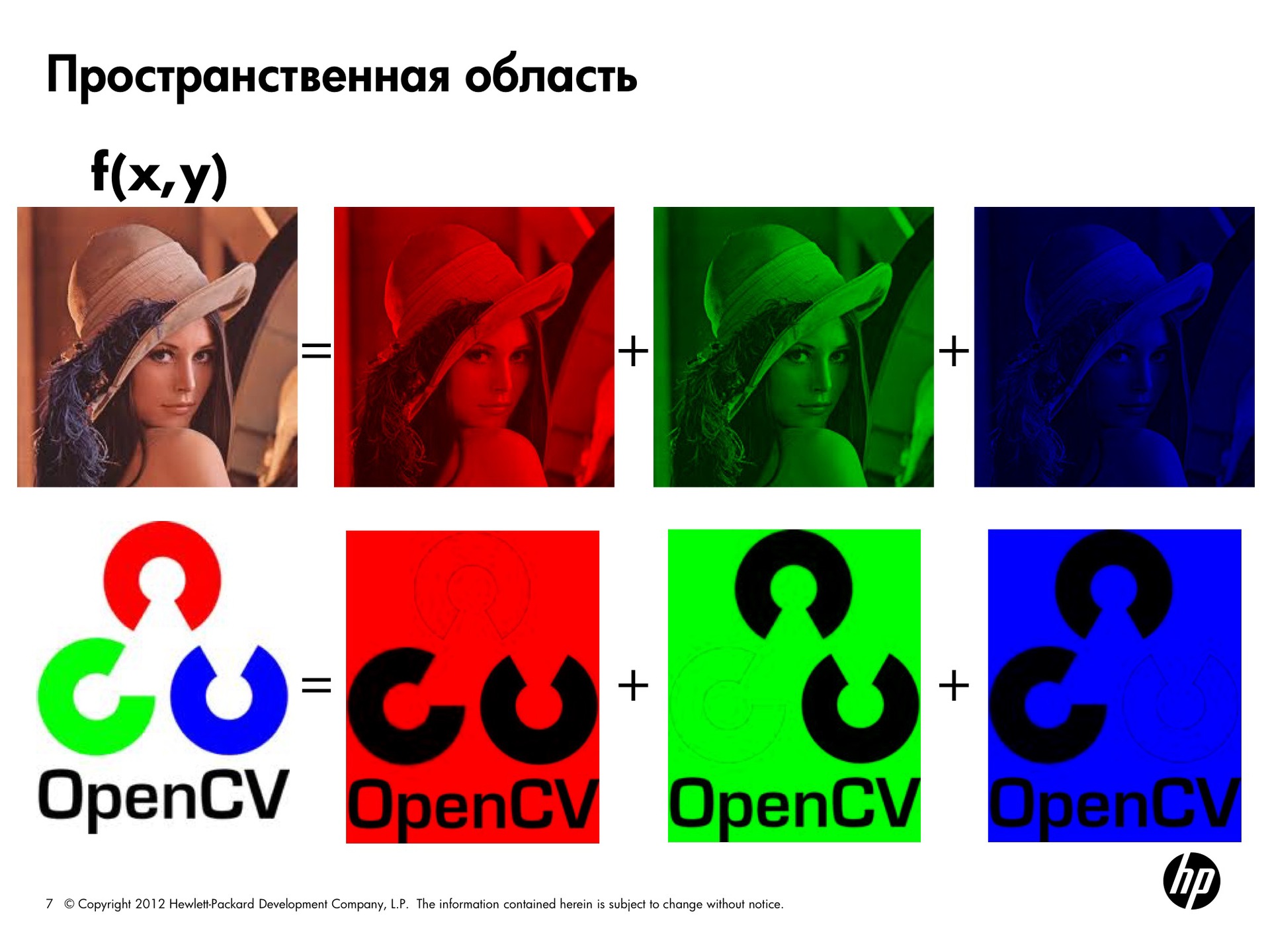
Recall that if there is no light source, we get a black color. If we combine the sources of all three primary colors, we get white. This means that in a darker area there is no convergence of a given color channel.
This is a familiar spatial representation. The following discussion will focus mainly on black and white pictures, but in principle all algorithms will be applicable to color images.
To simplify the task, imagine that our image is one-dimensional. The line, which goes from left to right, displays all changes in brightness. The splash at the beginning corresponds to a pair of white pixels, then there is a gray area, then a white one again. On black we fall down. That is, along this line, you can trace how the brightness changes.
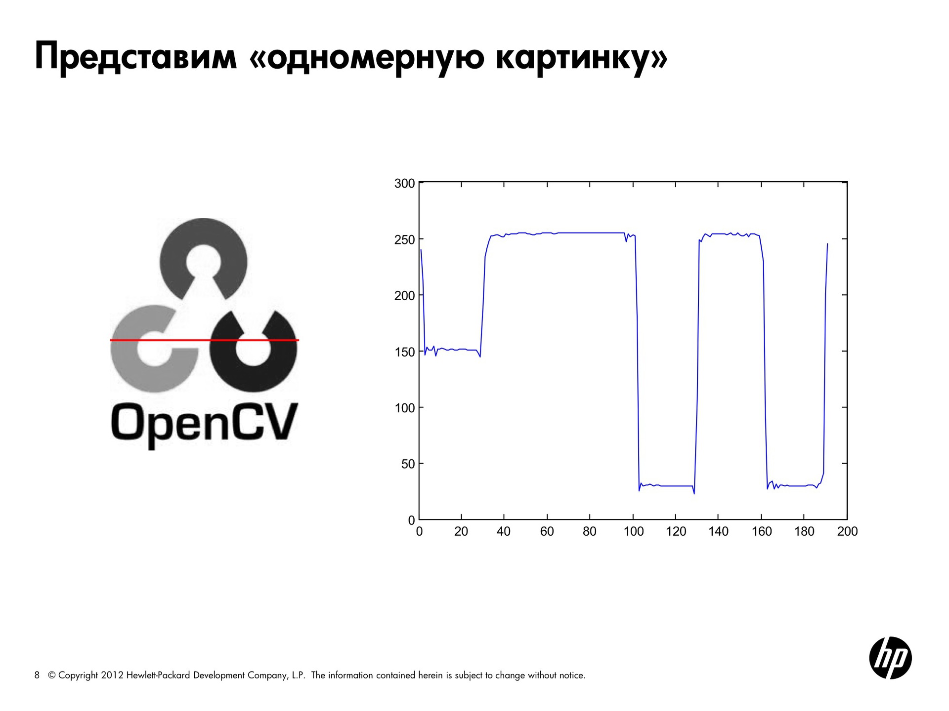
Let's see another example.
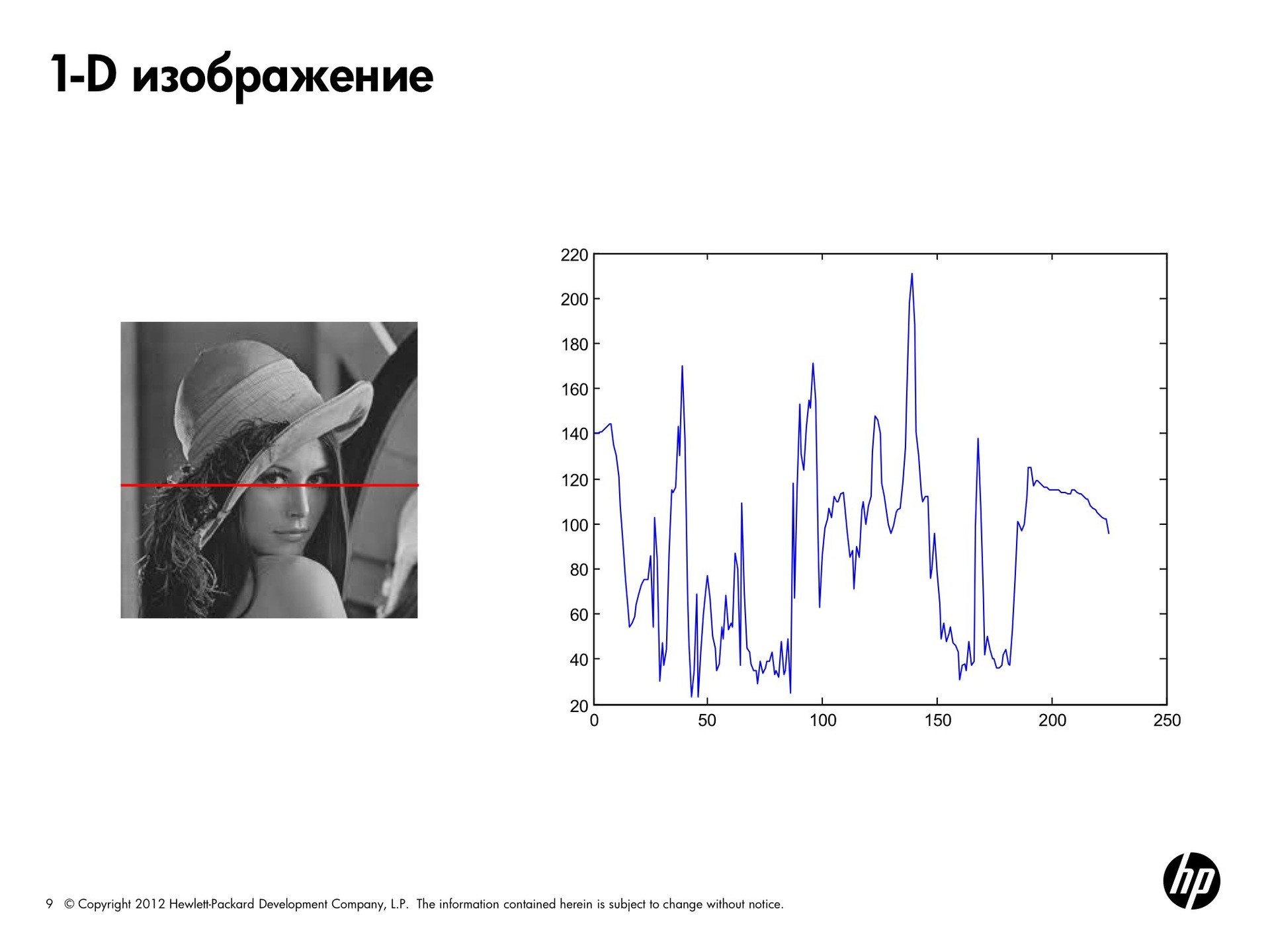
How else can you describe the information contained in our signal, in addition to data on its brightness? You can decompose it into components, that is, for example, very smooth the curve to track the overall trend. Here it goes down first, then up, then down again and up again. We get almost asymptotic approximation to this thing.
Then we can look at the details bigger, i.e. what are the bursts, the details are smaller. What I'm getting at is that: in principle, you can decompose this function into harmonic components. For those who remember that such a Fourier series, according to the theorem of the same name, any function (she said - periodic, but this is not true, in general, any function) can be represented as the sum of sines and cosines of various frequencies and amplitudes, which is shown here. This artificially generated function is the sum of these four functions.
What can we do about it? Imagine that we have a certain basis, which is given by a set of these sine waves and cosines. We know the frequency of each basic function. Then, to represent the original function, we need to know only the coefficients, the scalar, by which we need to multiply each of the basis functions.
The basic idea of the Fourier transform is that any picture can be represented as a sum of sines and cosines. Why any? Because any periodic function can always be represented as a sum of sines and cosines. The non-periodic function, if the area of the graph under it is finite (which will always be true for the image), can also be represented as the sum of a sine wave and cosines. To present such a function absolutely precisely, there must be infinitely many of them, but, nevertheless, this can be done.
The frequencies of such terms will characterize the image. For each picture we say which of the basic frequencies prevails in it.
What can we say about the coefficients of the basis functions? If we have a large coefficient before the base function with a high frequency, this means that the brightness changes quite often. The picture has a lot of brightness differences in small local regions. If the picture is described by smooth sinusoids, with a low frequency, then this means that there are many homogeneous areas in the picture, the brightness changes smoothly, or the picture, for example, has been “drilled”.
Thus, you can use the mapping in the frequency domain to describe the images.
We take the original signal, represent it as a sum of oscillations of the same amplitude and different frequencies, multiply them by rock coefficients and obtain the decomposition of the original function in this new basis.
Now imagine that you are trying to transfer a picture to someone using a mobile phone. Previously, you would need to transmit all 230 brightness values. But now, if the receiving and receiving side "know" what our basic functions are, then the volume of information sent is greatly reduced. You can pass the same information using significantly fewer parameters.
Why is the Fourier transform so popular in image processing? It allows you to significantly reduce the amount of transmitted information, sufficient to restore the image in its previous form. Also, the Fourier transform facilitates the filtering process, but more on that later. Fourier transform is good because it is reversible. We have decomposed our function into frequency components with coefficients, but we can go back and forth from the frequency to the spatial representation.
Theoretically, we can present a function as an infinite set of sinusoids, but in practice (since infinity is unattainable), they are limited to only a few first terms (with the largest coefficients). The picture will be slightly different from the original when restored back to the spatial area, that is, some of the information will be irretrievably lost. However, the use of a limited number of components allows you to sufficiently restore the image.
How to calculate the values of scalars for a predetermined frequency basis? For the Fourier transform, when we have harmonics, sines and cosines, as basic functions. And there is an inverse Fourier transform, which allows, by a set of coefficients depending on frequency, to reconstruct the original representation in the spatial domain.
Here harmonics are those sines and cosines that are drawn on the previous slide. For each fixed frequency, there is a function of x.
I hope that with the case of the same name more or less clear. Now let's look at the two-dimensional case, because the picture is two-dimensional.
Here we can also construct two-dimensional harmonics, which will already depend on four parameters: x, y (from two directions) and from two frequencies in the x and y directions, respectively.
Take, for example, such a square. Both the top view and the isomers are drawn here. We see how our harmonic smoothly moves from one corner to another. Here again we can apply the direct Fourier transform, and the opposite, where we already have coefficients for two fixed frequencies, in order to get a spatial representation again.
Now let's see what can be understood when visualizing the result of a direct transformation using the so-called Fourier spectrum. Although we are talking about the Fourier transform, we can also use any other signal transform, where we will choose not other harmonics as basis functions, but some other functions. Often, [wavelets] are used as basic functions. In a sense, they are more successful than sines and cosines.
Let's try to consider the hail from the values of our scalars. Here we have a discrete case - what the basic function looks like for fixed u and v. Arrange them along the axes u and v respectively. On this make-up, the Fourier spectrum is a display of the values of the coefficients. It is important to understand that in the center we have zero frequency, and it increases towards the edges.
Further, if each cell begins to add the value of the parameter F, the coefficient that we obtained during the decomposition. The larger the coefficient, the brighter it will be displayed on the spectrum. That is, we want to visualize the Fourier spectrum. If the coefficient is F = 0, we will display it in black. The bigger it is, the brighter the color.
On a two-dimensional spectrum, only one pixel will correspond to u = 0, v = 0, the next one will be U = -1, V = 0. The pixel value will be equal to the coefficient obtained from the transformation. It is important that the central coefficients correspond to the importance of this harmonic in the image representation, in the center there are harmonics with zero frequencies. That is, in the picture, if we have a very large response here, this means that the picture practically does not change its brightness. If the picture has a dark spot here, and there is a bright spot on the periphery, then it is colorful - there is a difference in brightness at each point and in each direction.
A picture is not a spectrum, it is a visualization of a two-dimensional sinusoid.
Let's look at this picture. Usually draw the logarithm of the spectrum, otherwise it turns out very dark. But for most of the pictures there is typically a bright spot in the center, because there are many homogeneous areas in the pictures. It should be borne in mind that when our frequency is zero, there is no difference in brightness. In case there is a difference in brightness, then to which point of the spectrum this difference will contribute will depend on the direction of the contour, on the direction of the differential. Here we have edges, but they are smeared on the periphery, there are no bright responses.
We turn to what you can do with images. Let's start with the simplest, intuitive transformations in the spatial domain.
If our brightness changes from 0 to 255, then for each pixel we write 255 minus its previous value. Black becomes white, and white becomes black.
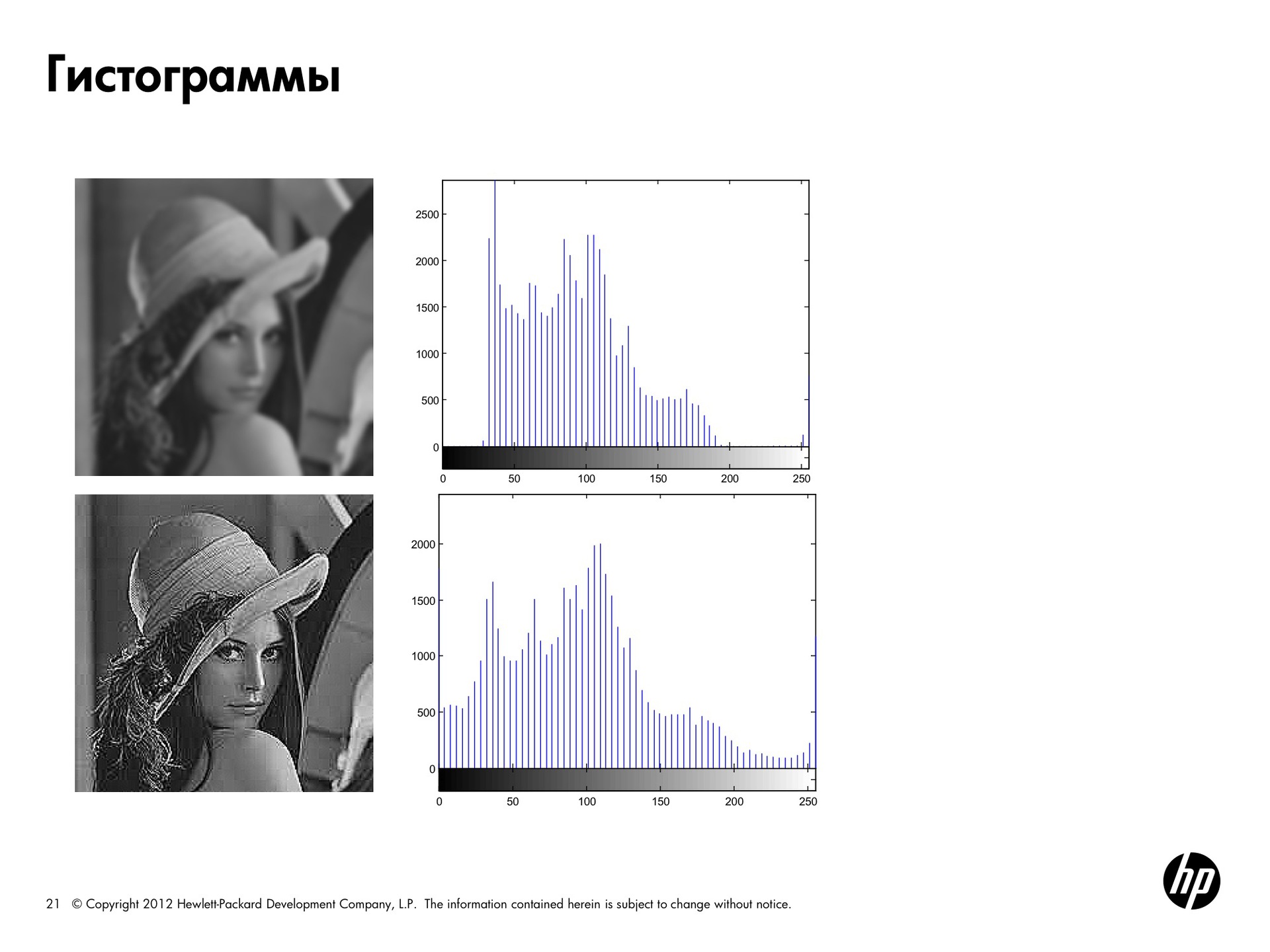
One of the most simple and practical types of image presentation is a histogram. For any image, you can calculate how many pixels are with zero brightness, how many with brightness of 50, 100, and so on, and get some sort of frequency distribution.
In this picture, Lena has all the points of brightness that are more than 125 cut off. We get a histogram shifted to the left and a dark picture. In the second picture, the opposite is true - there are only bright pixels, the histogram is shifted to the right.
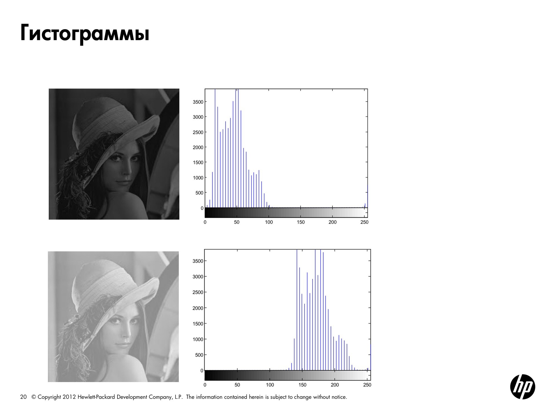
The next picture is smeared, it has no clear contours. Such a picture is characterized by a brightness column somewhere in the middle and the absence of energy at the edges of the spectrum.
For the second Lena, processing was done from this slide to emphasize each of the contours, that is, to make the brightness drops stronger. Here the histogram occupies the entire range of brightness.
What can you do with histograms? The shape of the histogram can already tell a lot about its properties. Then you can do something with the histogram, change its shape to make the picture look better.
For a dark picture, the histogram can be stretched to the right, and then the picture will become brighter, and for a light one, vice versa. This is true for any form. If the histogram of the picture does not cover the entire frequency range, then with uniform stretching the picture will become more contrast and details will be better seen.
We just made linear histogram transforms. You can do nonlinear transformations, which are called adaptation or linearization. This allows you to get a more uniform one from the original histogram with approximately the same number of pixels of each brightness.
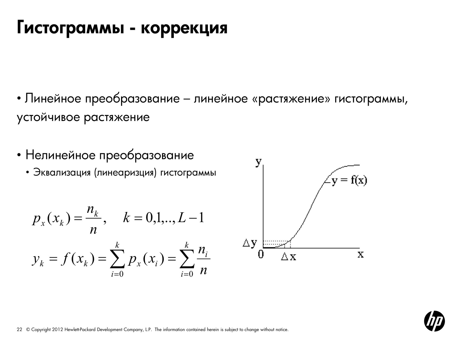
It is done this way. In the formula, x k is a certain level of brightness, n k is the number of pixels of such brightness, n is the total number of pixels. We choose a pixel and get the probability with which it will be the color x k . That is, the number of pixels n k divided by the total number of pixels. Actually - a share.
Let us try to obtain a uniform probability density, that is, for each color to have the same probability of obtaining it. This is achieved by the following conversion. If we calculate the new brightness values for it y k by the pixel of the color x k by the formula, that is, we take and enumerate all the probabilities from i to this color, the histogram will be more uniform. That is, the original darkened picture looked like this, and if we apply screen adaptation to the brightness of this picture, then we get a histogram of this form as a result. As you can see, they are much more evenly distributed across all possible values, and the picture will look like this.
Do the same for the bright picture. And the histograms practically coincide, because initially the pictures were obtained from the same picture.
Here are the results of equalization for sharp and blurry pictures. It can be seen that for a sharp picture the image has hardly changed, but the histogram has become a bit smoother.
We have already abandoned color images and are talking only about black and white, where there are various gradations of gray. Binarization is a continuation of the mockery of the image, when we also give up on them. As a result, we get a picture where there is only black and white. We need to understand which pixels we want to make black and which ones white.
This simplifies further image analysis for many tasks. If there is a picture with text, for example, it would be good if all the letters in the picture turned out to be white (or black), and the background is the other way around. A subsequent character recognition algorithm will make it easier to work with such an image. That is, binarization is good when we want to clearly separate the ph from the object.
Let's talk about the simplest type of binarization - the threshold one. This type is generally not very applicable for photographs, but, nevertheless, sometimes used.

If we apply threshold binarization to the histogram, we see that we have two types of pixels in the image: darker and lighter. It is usually assumed that a larger number of pixels corresponds to the background. From this we conclude that here we have a lot more, it is dark, respectively, we have a dark background, and it has one or more light objects. The object can be composite. Here we have two bright objects of different colors.
These are very beautiful histograms, in life you are unlikely to see such. But it is easy to understand from them where it is necessary to hold a threshold in order to separate the background from the object. Here, if we take the threshold value exactly between them, and all the pixels that are brighter than the threshold are made white, and those that are darker black, we will perfectly separate the object from the background. Having chosen the range of brightness we need, we cut one or another object out of the picture.
Binarization varies by type based on how the threshold is calculated. With global binarization, the threshold is the same for all image points. With local and dynamic binarization, the threshold depends on the coordinate of the point. With adaptive binarization, the threshold also depends on the brightness value at this point.
The choice of the threshold for global binarization is as follows. You can do it manually, but of course no one wants to do anything manually manually, but you can automatically select a threshold.
The simplest algorithm is as follows: first, take an arbitrary threshold value and segment the image along this threshold into two regions. One contains pixels with a value greater than the threshold, and the other less than the threshold. For these regions, we calculate the average brightness value. After that, we consider them a half-sum as a new threshold. The algorithm finishes its work when, after a certain number of iterations, the final brightness becomes less than one more specified threshold value.
This picture shows the advantage of local binarization.

If binarization were global, a global threshold for the whole picture would be chosen, the result would look like this in picture b. The pixels here are in one area at about the same brightness level, so the whole part turns out white, illuminated. In that case, if we apply the simplest version of local binarization — that is, divide the image into segments and choose the threshold for each segment separately — the result of binarization will already look better.
For this picture, the histogram is likely to be beautiful. There will be peaks, and in the valley, maybe there will not be a zero value. Here is a bright and dark area. That is, we chose a threshold, but it cannot be selected in such a way as to select this object, because if the threshold is one, then the criterion by which we make the pixel black or white is one for all pixels of the picture. The color is the same, with a single threshold, we can never carry them into different components.
If you want to binarize a complex picture, then you need to segment it well first. The easiest way is to apply a fixed grid. If you have an idea of how to segment, then you can choose a global threshold in each area and binarization will work.
In these two areas, everything is bad, because there are completely black pixels and there is - more light. For each square we find the threshold and apply it inside this square.
Suppose we have a binary image consisting of only black and white pixels. We want to mark the belonging of pixels to a connected area in this way: all the pixels inside a given area of the same color and are connected to each other.

Separate all connected whites from all blacks. There are four- and eight-connected domains. In four-connected neighbors, only pixels located vertically and horizontally are counted, and in eight-connected regions, diagonal neighbors are also taken into account.
The simplest algorithm is a two-pass, it works as follows. We start from the top left corner and assign a number to the first pixel. Next we move to the right and see if the color of the pixel coincides with the already marked one. If it is the same, then assign the same label to it. If this pixel was marked with a zero, then this one also gets a zero. And so we reach the end of the line, because here we have all zeroes. Further, the color of the third pixel on the second line does not match the color of the already marked neighbors. We increment the area counter and assign this pixel the number of the next region - 1. Go here, this neighbor already eats the same color that has a label, assign it the same label. Next we increase the counter and assign the numbers 2, 3, 4, 5, 6, 7. Here is the result of the first pass. In the second pass, we will only have to combine the areas in which neighbors of the same color wear different labels. The result is an image of this type.
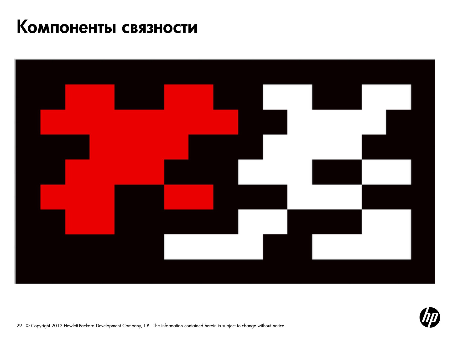
Here is the background of one color, one connected component of another, and the second connected component of a third color. Red and white components on a black background.
Already in the first pass, information accumulates that several labels correspond to one component. It is clear that they are all the same color and 1 and 2 belong to the same component. This information is recorded and is renumbered in the second pass.
Where is it used? This is one way to segmentation of a picture. The simplest example is when the picture is binary, you can select the components of connectivity in a color image. Only there the criterion of joining one component will not be full color matching, but the fact that they differ by some threshold value.
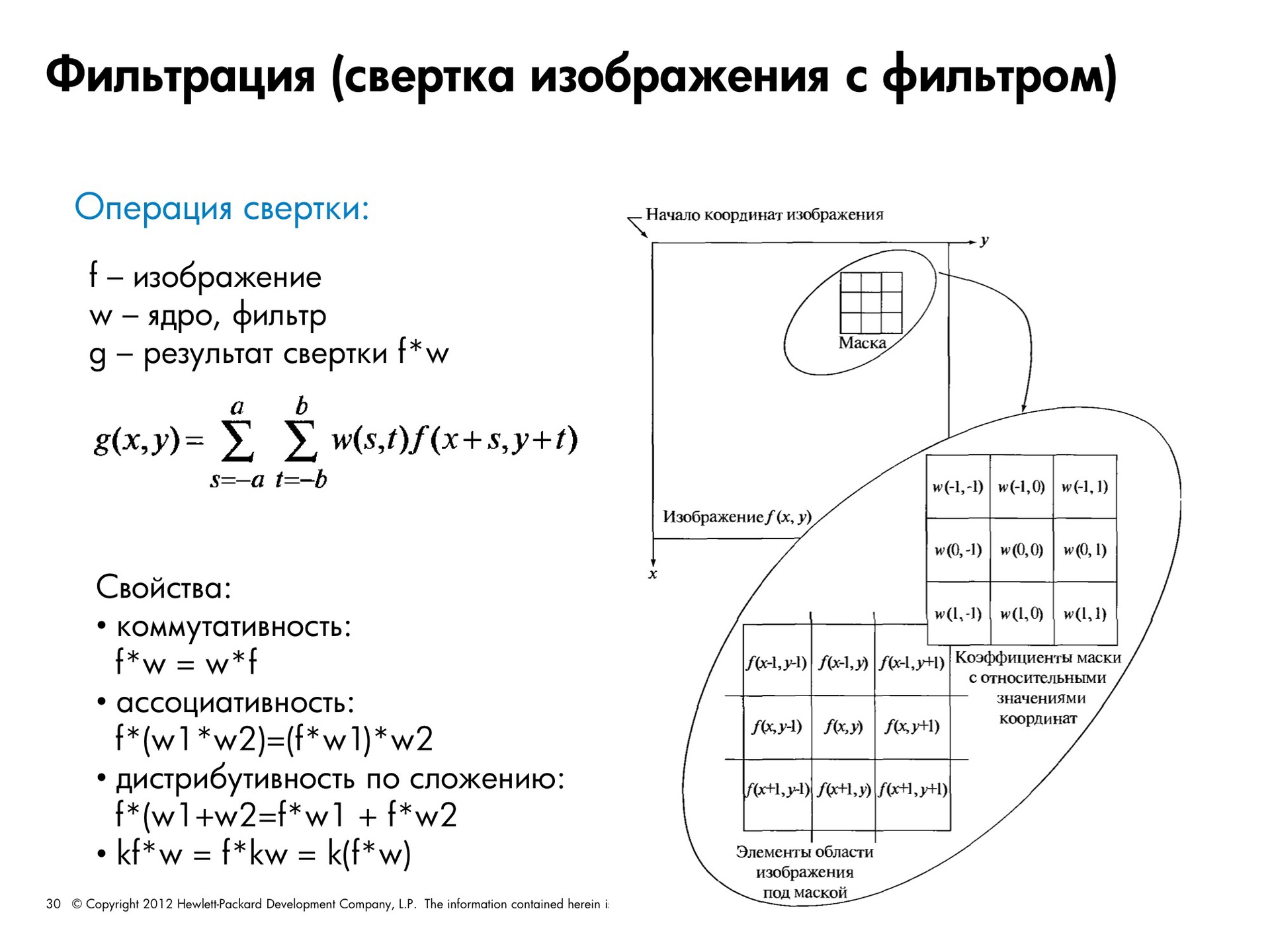
This is a more complex topic. In a nutshell, filtering is the application of a function to an image. The filtering operation is called convolution. It is performed as follows.
Imagine that we have a picture in the spatial domain and there is a filter (it is the mask, it is the core) —a certain function. In the discrete case, this is an array with values. We put this mask on a piece of the image. Then the value of the pixel located under the central element of the mask is calculated as the weighted sum of the pixel values multiplied by the mask values. That is, we impose a mask on the image and the value in the pixel, which is under the center, is calculated as the pixel value multiplied by the mask coefficient plus the value multiplied by the coefficient in another place and so on.
The mask slides over the picture, we must impose it on each of the pixels. With the border pixels, the following happens. In order to be able to filter, we choose two options: either the output image will be smaller than the original one, since it is cut to the size of the filter, that is, it will be cut off by half of the filter from above, below and from the sides. Or we increase the original image. Most often either black pixels are added, or more appropriately, mirrored pixels of the edge of the picture.
That is, if we have such a picture and such a filter (3 by 3), and if we do nothing with the picture, then only this part is filtered out. Lose one pixel on each side. We can increase the original image by one more pixel by inserting black or white pixels along the edges, or mirror reflecting the edge. If we have a larger filter, then we accordingly increase the area that is growing along the edge.
The convolution operation has a number of pleasant properties, such as commutativity, that is, no matter what comes first, an image or a filter. Associativity, that is, if we have two filters, we can either apply first and then the second, or build a convolution of filters based on these filters, and then apply it to the image.
Distribution by addition - we can add two filters, simply add their weights and get a new filter, or first apply one filter, then the second and add results. The scalar can be taken out of the brackets. That is, if there is a coefficient here, we can divide all weights by some number, apply a filter, and then multiply the result by this constant. What happens if we fold the picture with this filter? Shift by one pixel.
I promised to tell you why the Fourier theorem works so well in the frequency domain. There is a convolution theorem. What it is? The convolution theorem says that if we produce convolution in the spatial domain, this is the same thing as multiplying the results of the Fourier transform in the frequency domain. If there is a picture F and a filter H, and we will try to minimize them, it will be the same as making a transfer of a picture and a filter to the frequency domain. That is, to find for the image and filter the Fourier transform coefficients and multiply them together. And in the opposite direction. If we have multiplication in the spatial domain, this is the same as the convolution operation over the corresponding Fourier transform coefficients.
Of course, we can take a filter for use in our picture, and move it for a long time throughout the image, but this is quite a difficult computational task. It is much easier to produce a fast Fourier transform of the filter and the image.
The averaging filter is one of the most famous. It allows you to remove random noise. The matrix of this filter looks like this.
Filter smoothes the image. If we rearrange the coefficients a little differently, this will make the contours brighter horizontally and vertically, that is, leave the brightness differences.
When we have a core and it collapses with something, these are linear filters, there all operations are linear. There are also filters based on ordinal statistics. Here, instead of averaging the values of each pixel, the median is taken.
This filter will already be non-linear. Median filters are more resistant to emissions, strong deviations from average values, so median filters are much better able to cope with suppressing salt and pepper noise.
Another very common filter is the Gauss filter. This is a Gaussian bundle that looks like this. There is a dependence on the radius. Here is the representation of the filter in the spatial domain and its representation in the frequency domain. Is it possible by the type of filter characteristics to determine what it will do with the picture?
Recall the convolution theorem. We are going to multiply the image of our image with this one. What happens? We significantly cut the high frequencies, the image will be smoother. Here is the result of anti-aliasing.
The original image, the picture is smoothed by a Gaussian filter with = 1.4 of size 5 and = 2.8 with a size of 10. The larger the radius, the more blurred the picture turns out, although there is clearly no relationship between the size of the filter (the number of samples) and in practice does not make sense choose a big one with a small size.
Here we have a 3x3 filter size (small), if it is large, this means that we will not be able to reflect all the values. The unspoken rule - the size should be about 5-6. Smoothing should be used when there is noise and we want to get rid of it. That is, we are trying to average the value at each point, looking at the values of the neighbors, and if this is some kind of outlier, then we will remove this value.
It happens that it is necessary to highlight some detail in the image. This can also be done using a convolution with a kernel of another kind. For example, a bundle with such a core will allow you to select point features. Unfortunately, it is not very clearly visible here, but there is a defect in the image, a white dot. Here is the result of the convolution of this image with this filter, here is a white dot. And this is the result of binarization, there is also a white dot.
Why are there practically no such contours left here? The picture shows them very clearly. The point became clearly visible on the convolution, and the contours are practically invisible. Because the point is isolated and the value at the point above which the mask is located is much higher than everything around.
You can detect lines by changing a bit the look of the core. If we set the core of this kind, we will well detect horizontal lines, of this kind - at an angle of 45 °, vertical and -45 °. Here is an example of processing the original image, the core at -45 ° and binarization.
In general, the selection of contours and lines and points is the selection of point features. There are many selection algorithms, now we'll talk about their basics.
How to find the drop in brightness in the image. What is the brightness drop? This is when we had the pixels of the same color, and then became the pixels of a different color. If we look at the profile of the picture, at first it was all black, then - once, it became gray. Or it smoothly changed. That is, we have a jump or a drop in brightness. In order to select it, you can simply take a derivative. In flat values (where the brightness does not change), the derivative is 0. Where the brightness changes, the higher the differential, the greater the value of the derivative. The first derivative will allow you to select the area of smooth changes in brightness. There is such a thing as zero crossing line. If we calculate the values of the derivatives and combine them, then we can assume that the contour is located somewhere here at this point, where the imaginary straight line crosses this level.
How can you calculate the derivative in the picture and what is the gradient of the image? We look at how much our brightness varies along x and y.
, , , .
. x - . 1 . .
, , . , , — , , — , — .
, x y. , . , . , .
, . — . , , , , , . , , — , e — , , g — .
, , , — Mexican Hat.
. , , , . , . .
, , , .
- build histograms;
- understand what can be done with the image, changing its histogram;
- suppress noise, learn about its forms.
In addition, we will get to know what is the representation of the image in the spatial domain and what is meant by the representation of the image in the frequency domain.
It is impossible to improve images without understanding why you are doing this. There may be two goals: correct it so that it is as you like, or convert it so that the computer can easily calculate some of its signs and extract useful information.
Spatial region
Recall that a picture is represented as a function of x and y. If we are talking about a full-fledged image, then each value of this function is a three-digit number that represents a value for each of the color channels.
Representation of an image in a spatial domain is how we are used to understanding and seeing an image. There are x and y, and at each point we have some kind of intensity value or color channel value.
In this slide, Lena and the OpenCV library logo are decomposed into three color channels — red, green, and blue.
Recall that if there is no light source, we get a black color. If we combine the sources of all three primary colors, we get white. This means that in a darker area there is no convergence of a given color channel.
This is a familiar spatial representation. The following discussion will focus mainly on black and white pictures, but in principle all algorithms will be applicable to color images.
To simplify the task, imagine that our image is one-dimensional. The line, which goes from left to right, displays all changes in brightness. The splash at the beginning corresponds to a pair of white pixels, then there is a gray area, then a white one again. On black we fall down. That is, along this line, you can trace how the brightness changes.
Let's see another example.
How else can you describe the information contained in our signal, in addition to data on its brightness? You can decompose it into components, that is, for example, very smooth the curve to track the overall trend. Here it goes down first, then up, then down again and up again. We get almost asymptotic approximation to this thing.
Then we can look at the details bigger, i.e. what are the bursts, the details are smaller. What I'm getting at is that: in principle, you can decompose this function into harmonic components. For those who remember that such a Fourier series, according to the theorem of the same name, any function (she said - periodic, but this is not true, in general, any function) can be represented as the sum of sines and cosines of various frequencies and amplitudes, which is shown here. This artificially generated function is the sum of these four functions.
What can we do about it? Imagine that we have a certain basis, which is given by a set of these sine waves and cosines. We know the frequency of each basic function. Then, to represent the original function, we need to know only the coefficients, the scalar, by which we need to multiply each of the basis functions.
The basic idea of the Fourier transform is that any picture can be represented as a sum of sines and cosines. Why any? Because any periodic function can always be represented as a sum of sines and cosines. The non-periodic function, if the area of the graph under it is finite (which will always be true for the image), can also be represented as the sum of a sine wave and cosines. To present such a function absolutely precisely, there must be infinitely many of them, but, nevertheless, this can be done.
The frequencies of such terms will characterize the image. For each picture we say which of the basic frequencies prevails in it.
What can we say about the coefficients of the basis functions? If we have a large coefficient before the base function with a high frequency, this means that the brightness changes quite often. The picture has a lot of brightness differences in small local regions. If the picture is described by smooth sinusoids, with a low frequency, then this means that there are many homogeneous areas in the picture, the brightness changes smoothly, or the picture, for example, has been “drilled”.
Thus, you can use the mapping in the frequency domain to describe the images.
We take the original signal, represent it as a sum of oscillations of the same amplitude and different frequencies, multiply them by rock coefficients and obtain the decomposition of the original function in this new basis.
Now imagine that you are trying to transfer a picture to someone using a mobile phone. Previously, you would need to transmit all 230 brightness values. But now, if the receiving and receiving side "know" what our basic functions are, then the volume of information sent is greatly reduced. You can pass the same information using significantly fewer parameters.
Why is the Fourier transform so popular in image processing? It allows you to significantly reduce the amount of transmitted information, sufficient to restore the image in its previous form. Also, the Fourier transform facilitates the filtering process, but more on that later. Fourier transform is good because it is reversible. We have decomposed our function into frequency components with coefficients, but we can go back and forth from the frequency to the spatial representation.
Theoretically, we can present a function as an infinite set of sinusoids, but in practice (since infinity is unattainable), they are limited to only a few first terms (with the largest coefficients). The picture will be slightly different from the original when restored back to the spatial area, that is, some of the information will be irretrievably lost. However, the use of a limited number of components allows you to sufficiently restore the image.
How to calculate the values of scalars for a predetermined frequency basis? For the Fourier transform, when we have harmonics, sines and cosines, as basic functions. And there is an inverse Fourier transform, which allows, by a set of coefficients depending on frequency, to reconstruct the original representation in the spatial domain.
Here harmonics are those sines and cosines that are drawn on the previous slide. For each fixed frequency, there is a function of x.
I hope that with the case of the same name more or less clear. Now let's look at the two-dimensional case, because the picture is two-dimensional.
Here we can also construct two-dimensional harmonics, which will already depend on four parameters: x, y (from two directions) and from two frequencies in the x and y directions, respectively.
Take, for example, such a square. Both the top view and the isomers are drawn here. We see how our harmonic smoothly moves from one corner to another. Here again we can apply the direct Fourier transform, and the opposite, where we already have coefficients for two fixed frequencies, in order to get a spatial representation again.
Now let's see what can be understood when visualizing the result of a direct transformation using the so-called Fourier spectrum. Although we are talking about the Fourier transform, we can also use any other signal transform, where we will choose not other harmonics as basis functions, but some other functions. Often, [wavelets] are used as basic functions. In a sense, they are more successful than sines and cosines.
Let's try to consider the hail from the values of our scalars. Here we have a discrete case - what the basic function looks like for fixed u and v. Arrange them along the axes u and v respectively. On this make-up, the Fourier spectrum is a display of the values of the coefficients. It is important to understand that in the center we have zero frequency, and it increases towards the edges.
Further, if each cell begins to add the value of the parameter F, the coefficient that we obtained during the decomposition. The larger the coefficient, the brighter it will be displayed on the spectrum. That is, we want to visualize the Fourier spectrum. If the coefficient is F = 0, we will display it in black. The bigger it is, the brighter the color.
On a two-dimensional spectrum, only one pixel will correspond to u = 0, v = 0, the next one will be U = -1, V = 0. The pixel value will be equal to the coefficient obtained from the transformation. It is important that the central coefficients correspond to the importance of this harmonic in the image representation, in the center there are harmonics with zero frequencies. That is, in the picture, if we have a very large response here, this means that the picture practically does not change its brightness. If the picture has a dark spot here, and there is a bright spot on the periphery, then it is colorful - there is a difference in brightness at each point and in each direction.
A picture is not a spectrum, it is a visualization of a two-dimensional sinusoid.
Let's look at this picture. Usually draw the logarithm of the spectrum, otherwise it turns out very dark. But for most of the pictures there is typically a bright spot in the center, because there are many homogeneous areas in the pictures. It should be borne in mind that when our frequency is zero, there is no difference in brightness. In case there is a difference in brightness, then to which point of the spectrum this difference will contribute will depend on the direction of the contour, on the direction of the differential. Here we have edges, but they are smeared on the periphery, there are no bright responses.
Processing in the spatial domain
We turn to what you can do with images. Let's start with the simplest, intuitive transformations in the spatial domain.
Invert picture
If our brightness changes from 0 to 255, then for each pixel we write 255 minus its previous value. Black becomes white, and white becomes black.
One of the most simple and practical types of image presentation is a histogram. For any image, you can calculate how many pixels are with zero brightness, how many with brightness of 50, 100, and so on, and get some sort of frequency distribution.
In this picture, Lena has all the points of brightness that are more than 125 cut off. We get a histogram shifted to the left and a dark picture. In the second picture, the opposite is true - there are only bright pixels, the histogram is shifted to the right.
The next picture is smeared, it has no clear contours. Such a picture is characterized by a brightness column somewhere in the middle and the absence of energy at the edges of the spectrum.
For the second Lena, processing was done from this slide to emphasize each of the contours, that is, to make the brightness drops stronger. Here the histogram occupies the entire range of brightness.
What can you do with histograms? The shape of the histogram can already tell a lot about its properties. Then you can do something with the histogram, change its shape to make the picture look better.
For a dark picture, the histogram can be stretched to the right, and then the picture will become brighter, and for a light one, vice versa. This is true for any form. If the histogram of the picture does not cover the entire frequency range, then with uniform stretching the picture will become more contrast and details will be better seen.
We just made linear histogram transforms. You can do nonlinear transformations, which are called adaptation or linearization. This allows you to get a more uniform one from the original histogram with approximately the same number of pixels of each brightness.
It is done this way. In the formula, x k is a certain level of brightness, n k is the number of pixels of such brightness, n is the total number of pixels. We choose a pixel and get the probability with which it will be the color x k . That is, the number of pixels n k divided by the total number of pixels. Actually - a share.
Let us try to obtain a uniform probability density, that is, for each color to have the same probability of obtaining it. This is achieved by the following conversion. If we calculate the new brightness values for it y k by the pixel of the color x k by the formula, that is, we take and enumerate all the probabilities from i to this color, the histogram will be more uniform. That is, the original darkened picture looked like this, and if we apply screen adaptation to the brightness of this picture, then we get a histogram of this form as a result. As you can see, they are much more evenly distributed across all possible values, and the picture will look like this.
Do the same for the bright picture. And the histograms practically coincide, because initially the pictures were obtained from the same picture.
Here are the results of equalization for sharp and blurry pictures. It can be seen that for a sharp picture the image has hardly changed, but the histogram has become a bit smoother.
Binarization
We have already abandoned color images and are talking only about black and white, where there are various gradations of gray. Binarization is a continuation of the mockery of the image, when we also give up on them. As a result, we get a picture where there is only black and white. We need to understand which pixels we want to make black and which ones white.
This simplifies further image analysis for many tasks. If there is a picture with text, for example, it would be good if all the letters in the picture turned out to be white (or black), and the background is the other way around. A subsequent character recognition algorithm will make it easier to work with such an image. That is, binarization is good when we want to clearly separate the ph from the object.
Let's talk about the simplest type of binarization - the threshold one. This type is generally not very applicable for photographs, but, nevertheless, sometimes used.
If we apply threshold binarization to the histogram, we see that we have two types of pixels in the image: darker and lighter. It is usually assumed that a larger number of pixels corresponds to the background. From this we conclude that here we have a lot more, it is dark, respectively, we have a dark background, and it has one or more light objects. The object can be composite. Here we have two bright objects of different colors.
These are very beautiful histograms, in life you are unlikely to see such. But it is easy to understand from them where it is necessary to hold a threshold in order to separate the background from the object. Here, if we take the threshold value exactly between them, and all the pixels that are brighter than the threshold are made white, and those that are darker black, we will perfectly separate the object from the background. Having chosen the range of brightness we need, we cut one or another object out of the picture.
Binarization varies by type based on how the threshold is calculated. With global binarization, the threshold is the same for all image points. With local and dynamic binarization, the threshold depends on the coordinate of the point. With adaptive binarization, the threshold also depends on the brightness value at this point.
The choice of the threshold for global binarization is as follows. You can do it manually, but of course no one wants to do anything manually manually, but you can automatically select a threshold.
The simplest algorithm is as follows: first, take an arbitrary threshold value and segment the image along this threshold into two regions. One contains pixels with a value greater than the threshold, and the other less than the threshold. For these regions, we calculate the average brightness value. After that, we consider them a half-sum as a new threshold. The algorithm finishes its work when, after a certain number of iterations, the final brightness becomes less than one more specified threshold value.
This picture shows the advantage of local binarization.
If binarization were global, a global threshold for the whole picture would be chosen, the result would look like this in picture b. The pixels here are in one area at about the same brightness level, so the whole part turns out white, illuminated. In that case, if we apply the simplest version of local binarization — that is, divide the image into segments and choose the threshold for each segment separately — the result of binarization will already look better.
For this picture, the histogram is likely to be beautiful. There will be peaks, and in the valley, maybe there will not be a zero value. Here is a bright and dark area. That is, we chose a threshold, but it cannot be selected in such a way as to select this object, because if the threshold is one, then the criterion by which we make the pixel black or white is one for all pixels of the picture. The color is the same, with a single threshold, we can never carry them into different components.
If you want to binarize a complex picture, then you need to segment it well first. The easiest way is to apply a fixed grid. If you have an idea of how to segment, then you can choose a global threshold in each area and binarization will work.
In these two areas, everything is bad, because there are completely black pixels and there is - more light. For each square we find the threshold and apply it inside this square.
Selection of connectivity components
Suppose we have a binary image consisting of only black and white pixels. We want to mark the belonging of pixels to a connected area in this way: all the pixels inside a given area of the same color and are connected to each other.
Separate all connected whites from all blacks. There are four- and eight-connected domains. In four-connected neighbors, only pixels located vertically and horizontally are counted, and in eight-connected regions, diagonal neighbors are also taken into account.
The simplest algorithm is a two-pass, it works as follows. We start from the top left corner and assign a number to the first pixel. Next we move to the right and see if the color of the pixel coincides with the already marked one. If it is the same, then assign the same label to it. If this pixel was marked with a zero, then this one also gets a zero. And so we reach the end of the line, because here we have all zeroes. Further, the color of the third pixel on the second line does not match the color of the already marked neighbors. We increment the area counter and assign this pixel the number of the next region - 1. Go here, this neighbor already eats the same color that has a label, assign it the same label. Next we increase the counter and assign the numbers 2, 3, 4, 5, 6, 7. Here is the result of the first pass. In the second pass, we will only have to combine the areas in which neighbors of the same color wear different labels. The result is an image of this type.
Here is the background of one color, one connected component of another, and the second connected component of a third color. Red and white components on a black background.
Already in the first pass, information accumulates that several labels correspond to one component. It is clear that they are all the same color and 1 and 2 belong to the same component. This information is recorded and is renumbered in the second pass.
Where is it used? This is one way to segmentation of a picture. The simplest example is when the picture is binary, you can select the components of connectivity in a color image. Only there the criterion of joining one component will not be full color matching, but the fact that they differ by some threshold value.
Filtering algorithms
This is a more complex topic. In a nutshell, filtering is the application of a function to an image. The filtering operation is called convolution. It is performed as follows.
Imagine that we have a picture in the spatial domain and there is a filter (it is the mask, it is the core) —a certain function. In the discrete case, this is an array with values. We put this mask on a piece of the image. Then the value of the pixel located under the central element of the mask is calculated as the weighted sum of the pixel values multiplied by the mask values. That is, we impose a mask on the image and the value in the pixel, which is under the center, is calculated as the pixel value multiplied by the mask coefficient plus the value multiplied by the coefficient in another place and so on.
The mask slides over the picture, we must impose it on each of the pixels. With the border pixels, the following happens. In order to be able to filter, we choose two options: either the output image will be smaller than the original one, since it is cut to the size of the filter, that is, it will be cut off by half of the filter from above, below and from the sides. Or we increase the original image. Most often either black pixels are added, or more appropriately, mirrored pixels of the edge of the picture.
That is, if we have such a picture and such a filter (3 by 3), and if we do nothing with the picture, then only this part is filtered out. Lose one pixel on each side. We can increase the original image by one more pixel by inserting black or white pixels along the edges, or mirror reflecting the edge. If we have a larger filter, then we accordingly increase the area that is growing along the edge.
The convolution operation has a number of pleasant properties, such as commutativity, that is, no matter what comes first, an image or a filter. Associativity, that is, if we have two filters, we can either apply first and then the second, or build a convolution of filters based on these filters, and then apply it to the image.
Distribution by addition - we can add two filters, simply add their weights and get a new filter, or first apply one filter, then the second and add results. The scalar can be taken out of the brackets. That is, if there is a coefficient here, we can divide all weights by some number, apply a filter, and then multiply the result by this constant. What happens if we fold the picture with this filter? Shift by one pixel.
I promised to tell you why the Fourier theorem works so well in the frequency domain. There is a convolution theorem. What it is? The convolution theorem says that if we produce convolution in the spatial domain, this is the same thing as multiplying the results of the Fourier transform in the frequency domain. If there is a picture F and a filter H, and we will try to minimize them, it will be the same as making a transfer of a picture and a filter to the frequency domain. That is, to find for the image and filter the Fourier transform coefficients and multiply them together. And in the opposite direction. If we have multiplication in the spatial domain, this is the same as the convolution operation over the corresponding Fourier transform coefficients.
Of course, we can take a filter for use in our picture, and move it for a long time throughout the image, but this is quite a difficult computational task. It is much easier to produce a fast Fourier transform of the filter and the image.
What can be filters / kernels and what they do with the image
The averaging filter is one of the most famous. It allows you to remove random noise. The matrix of this filter looks like this.
Filter smoothes the image. If we rearrange the coefficients a little differently, this will make the contours brighter horizontally and vertically, that is, leave the brightness differences.
When we have a core and it collapses with something, these are linear filters, there all operations are linear. There are also filters based on ordinal statistics. Here, instead of averaging the values of each pixel, the median is taken.
This filter will already be non-linear. Median filters are more resistant to emissions, strong deviations from average values, so median filters are much better able to cope with suppressing salt and pepper noise.
Another very common filter is the Gauss filter. This is a Gaussian bundle that looks like this. There is a dependence on the radius. Here is the representation of the filter in the spatial domain and its representation in the frequency domain. Is it possible by the type of filter characteristics to determine what it will do with the picture?
Recall the convolution theorem. We are going to multiply the image of our image with this one. What happens? We significantly cut the high frequencies, the image will be smoother. Here is the result of anti-aliasing.
The original image, the picture is smoothed by a Gaussian filter with = 1.4 of size 5 and = 2.8 with a size of 10. The larger the radius, the more blurred the picture turns out, although there is clearly no relationship between the size of the filter (the number of samples) and in practice does not make sense choose a big one with a small size.
Here we have a 3x3 filter size (small), if it is large, this means that we will not be able to reflect all the values. The unspoken rule - the size should be about 5-6. Smoothing should be used when there is noise and we want to get rid of it. That is, we are trying to average the value at each point, looking at the values of the neighbors, and if this is some kind of outlier, then we will remove this value.
It happens that it is necessary to highlight some detail in the image. This can also be done using a convolution with a kernel of another kind. For example, a bundle with such a core will allow you to select point features. Unfortunately, it is not very clearly visible here, but there is a defect in the image, a white dot. Here is the result of the convolution of this image with this filter, here is a white dot. And this is the result of binarization, there is also a white dot.
Why are there practically no such contours left here? The picture shows them very clearly. The point became clearly visible on the convolution, and the contours are practically invisible. Because the point is isolated and the value at the point above which the mask is located is much higher than everything around.
You can detect lines by changing a bit the look of the core. If we set the core of this kind, we will well detect horizontal lines, of this kind - at an angle of 45 °, vertical and -45 °. Here is an example of processing the original image, the core at -45 ° and binarization.
In general, the selection of contours and lines and points is the selection of point features. There are many selection algorithms, now we'll talk about their basics.
How to find the drop in brightness in the image. What is the brightness drop? This is when we had the pixels of the same color, and then became the pixels of a different color. If we look at the profile of the picture, at first it was all black, then - once, it became gray. Or it smoothly changed. That is, we have a jump or a drop in brightness. In order to select it, you can simply take a derivative. In flat values (where the brightness does not change), the derivative is 0. Where the brightness changes, the higher the differential, the greater the value of the derivative. The first derivative will allow you to select the area of smooth changes in brightness. There is such a thing as zero crossing line. If we calculate the values of the derivatives and combine them, then we can assume that the contour is located somewhere here at this point, where the imaginary straight line crosses this level.
How can you calculate the derivative in the picture and what is the gradient of the image? We look at how much our brightness varies along x and y.
, , , .
. x - . 1 . .
, , . , , — , , — , — .
, x y. , . , . , .
, . — . , , , , , . , , — , e — , , g — .
, , , — Mexican Hat.
. , , , . , . .
, , , .
Source: https://habr.com/ru/post/254249/
All Articles