Very large postgres

It just so happened that recently I had to deal with optimization and scaling of various systems. One of the tasks was scaling PostgreSQL. How does DB optimization usually occur? Probably, first of all, they look at how to choose the optimal settings for work and what indices can be created. If we didn’t do a little with blood, we’ve transferred to increasing server capacity, moving log files to a separate disk, load balancing, partitioning tables into partitions, and all kinds of refactoring and model redesign. And now everything is perfectly tuned, but there comes a time when all these movements are not enough. What to do next? Horizontal scaling and sharding data.



I want to share my experience in deploying a horizontally scalable cluster on a Postgres-XL database.

Postgres-XL is an excellent tool that allows you to combine several PostgreSQL clusters in such a way that they work as a single instance DB. For a client that connects to the database, there is no difference whether it works with a single PostgreSQL instance or with a Postgres-XL cluster. Postgres-XL offers 2 modes of spreading tables across a cluster: replication and sharding. During replication, all nodes contain the same copy of the table, and when sharding, data is evenly distributed among the cluster members. The current implementation is based on PostgreSQL-9.2. So almost all features of version 9.2 will be available to you.
')

Terminology

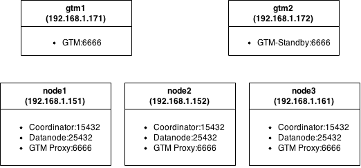
Postgres-XL consists of three types of components: global transaction monitor ( GTM ), coordinator (coordinator) and data node (datanode).

GTM is responsible for enforcing ACID requirements. Responsible for issuing identifiers. Since it is a single point of failure, it is recommended to prop up using GTM Standby. Dedicating a separate server for GTM is a good idea. To merge multiple requests and responses from coordinators and data nodes running on the same server, it makes sense to configure GTM-Proxy. This reduces the load on GTM as the total number of interactions with it decreases.

The coordinator is the central part of the cluster. It is with him that the client application interacts. Manages user sessions and interacts with GTM and data nodes. Parse requests, builds a query execution plan and sends it to each of the components involved in the request, collects the results and sends them back to the client. The coordinator does not store any user data. It stores only the service data to determine how to handle queries, where the data nodes are located. If one of the coordinators fails, you can simply switch to another.

The data node is the place where user data and indexes are stored. Communication with data nodes is carried out only through coordinators. For high availability, you can back up each stanby node with a server.



Pgpool-II can be used as a load balancer. It has already been discussed a lot on its configuration, for example, here and here It’s good practice to install a coordinator and a data node on one machine, since we don’t need to worry about load balancing and data from replicated tables can be obtained on site without sending an additional request over the network.

Test cluster layout

Each node is a virtual machine with modest hardware: MemTotal: 501284 kB, cpu MHz: 2604.

Installation

Everything is standard here: download the source from offsite , deliver dependencies, compile. Collected on Ubuntu server 14.10.

$ sudo apt-get install flex bison docbook-dsssl jade iso8879 docbook libreadline-dev zlib1g-dev $ ./configure --prefix=/home/${USER}/Develop/utils/postgres-xl --disable-rpath $ make world 

After the package is assembled, we upload it to the cluster nodes and proceed to setting up the components.

GTM customization

To ensure fault tolerance, consider an example with setting up two GTM servers. On both servers we create a working directory for GTM and initialize it.

 $ mkdir ~/gtm $ initgtm -Z gtm -D ~/gtm/ 

Then go to configuring configs:

gtm1

gtm2

Save, start:

 $ gtm_ctl start -Z gtm -D ~/gtm/ 

In the logs we observe records:
LOG: Started to run as GTM-Active.
LOG: Started to run as GTM-Standby.

GTM-Proxy Setup

 $ mkdir gtm_proxy $ initgtm -Z gtm_proxy -D ~/gtm_proxy/ $ nano gtm_proxy/gtm_proxy.conf 

After editing the config, you can run:

 $ gtm_ctl start -Z gtm_proxy -D ~/gtm_proxy/ 

Setting up coordinators

 $ mkdir coordinator $ initdb -D ~/coordinator/ -E UTF8 --locale=C -U postgres -W --nodename coordinator1 $ nano ~/coordinator/postgresql.conf 

Data node setup

 $ mkdir ~/datanode $ initdb -D ~/datanode/ -E UTF8 --locale=C -U postgres -W --nodename datanode1 $ nano ~/datanode/postgresql.conf 

For the remaining nodes, the setting is different only by specifying a different name.
Now rule pg_hba.conf:

 echo "host all all 192.168.1.0/24 trust" >> ~/datanode/pg_hba.conf echo "host all all 192.168.1.0/24 trust" >> ~/coordinator/pg_hba.conf 

Run and Tune-up

Everything is ready and can be run.

 $ pg_ctl start -Z datanode -D ~/datanode/ -l ~/datanode/datanode.log $ pg_ctl start -Z coordinator -D ~/coordinator/ -l ~/coordinator/coordinator.log 

We go to the coordinator:

 psql -p15432 

Execute the query:

 select * from pgxc_node; 

The request shows how the current server sees our cluster.
Example output:

  node_name | node_type | node_port | node_host | nodeis_primary | nodeis_preferred | node_id -------------+-----------+-----------+-----------+----------------+------------------+------------ coordinator1 | C | 5432 | localhost | f | f | 1938253334 

These settings are incorrect and can be safely removed.

 delete from pgxc_node; 

Create a new display of our cluster:

 create node coordinator1 with (type=coordinator, host='192.168.1.151', port=15432); create node coordinator2 with (type=coordinator, host='192.168.1.152', port=15432); create node coordinator3 with (type=coordinator, host='192.168.1.161', port=15432); create node datanode1 with (type=datanode, host='192.168.1.151', primary=true, port=25432); create node datanode2 with (type=datanode, host='192.168.1.152', primary=false, port=25432); create node datanode3 with (type=datanode, host='192.168.1.161', primary=false, port=25432); SELECT pgxc_pool_reload(); select * from pgxc_node; node_name | node_type | node_port | node_host | nodeis_primary | nodeis_preferred | node_id --------------+-----------+-----------+---------------+----------------+------------------+------------- datanode1 | D | 25432 | 192.168.1.151 | t | f | 888802358 coordinator1 | C | 15432 | 192.168.1.151 | f | f | 1938253334 coordinator2 | C | 15432 | 192.168.1.152 | f | f | -2089598990 coordinator3 | C | 15432 | 192.168.1.161 | f | f | -1483147149 datanode2 | D | 25432 | 192.168.1.152 | f | f | -905831925 datanode3 | D | 25432 | 192.168.1.161 | f | f | -1894792127 

On the remaining nodes you need to do the same.
The data node will not completely clear the information, but you can overwrite it:

 psql -p 25432 -c "alter node datanode1 WITH ( TYPE=datanode, HOST ='192.168.1.151', PORT=25432, PRIMARY=true);" 

Cluster testing

Now everything is set up and working. Create several test tables.

 CREATE TABLE test1 ( id bigint NOT NULL, profile bigint NOT NULL, status integer NOT NULL, switch_date timestamp without time zone NOT NULL, CONSTRAINT test1_id_pkey PRIMARY KEY (id) ) to node (datanode1, datanode2); CREATE TABLE test2 ( id bigint NOT NULL, profile bigint NOT NULL, status integer NOT NULL, switch_date timestamp without time zone NOT NULL, CONSTRAINT test2_id_pkey PRIMARY KEY (id) ) distribute by REPLICATION; CREATE TABLE test3 ( id bigint NOT NULL, profile bigint NOT NULL, status integer NOT NULL, switch_date timestamp without time zone NOT NULL, CONSTRAINT test3_id_pkey PRIMARY KEY (id) ) distribute by HASH(id); CREATE TABLE test4 ( id bigint NOT NULL, profile bigint NOT NULL, status integer NOT NULL, switch_date timestamp without time zone NOT NULL ) distribute by MODULO(status); 

It was created 4 tables with the same structure, but different distribution logic across the cluster.

The data from the test1 table will be stored only on 2x data nodes - datanode1 and datanode2 , and they will be distributed using the roundrobin algorithm. The remaining tables involve all nodes. Table test2 works in replication mode. To determine on which server the data of the test3 table will be stored, the hash function is used by the id field, and to determine the distribution logic of test4, the module is taken by the status field. Now let's try to fill them:

 insert into test1 (id, profile, status, switch_date) select a, round(random()*10000), round(random()*4), now() - '1 year'::interval * round(random() * 40) from generate_series(1,10) a; insert into test2 (id , profile,status, switch_date) select a, round(random()*10000), round(random()*4), now() - '1 year'::interval * round(random() * 40) from generate_series(1,10) a; insert into test3 (id , profile,status, switch_date) select a, round(random()*10000), round(random()*4), now() - '1 year'::interval * round(random() * 40) from generate_series(1,10) a; insert into test4 (id , profile,status, switch_date) select a, round(random()*10000), round(random()*4), now() - '1 year'::interval * round(random() * 40) from generate_series(1,10) a; 

Now we will request this data and see how the scheduler works.

 explain analyze select count(*) from test1; QUERY PLAN ------------------------------------------------------------------------------------------------------------------------------------- Aggregate (cost=27.50..27.51 rows=1 width=0) (actual time=0.649..0.649 rows=1 loops=1) -> Remote Subquery Scan on all (datanode1,datanode2) (cost=0.00..24.00 rows=1400 width=0) (actual time=0.248..0.635 rows=2 loops=1) Total runtime: 3.177 ms explain analyze select count(*) from test2; QUERY PLAN ------------------------------------------------------------------------------------------------------------------------------------- Remote Subquery Scan on all (datanode2) (cost=27.50..27.51 rows=1 width=0) (actual time=0.711..0.711 rows=1 loops=1) Total runtime: 2.833 ms explain analyze select count(*) from test3; QUERY PLAN ------------------------------------------------------------------------------------------------------------------------------------- Aggregate (cost=27.50..27.51 rows=1 width=0) (actual time=1.453..1.453 rows=1 loops=1) -> Remote Subquery Scan on all (datanode1,datanode2,datanode3) (cost=0.00..24.00 rows=1400 width=0) (actual time=0.465..1.430 rows=3 loops=1) Total runtime: 3.014 ms 

The scheduler tells us how many nodes will participate in the request. Since table2 replicates to all nodes, only 1 node will be scanned. By the way, it is unclear by what logic it is selected. It would be logical for him to request data from the same node on which the coordinator is.

By connecting to the data node (on port 25432) you can see how the data was distributed.

Now let's try to fill the tables with large amounts of data and compare query performance with standalone PostgreSQL.

 insert into test3 (id , profile,status, switch_date) select a, round(random()*10000), round(random()*4), now() - '1 year'::interval * round(random() * 40) from generate_series(1,1000000) a; 

Query in a Postgres-XL cluster:

 explain analyze select profile, count(status) from test3 where status<>2 and switch_date between '1970-01-01' and '2015-01-01' group by profile; QUERY PLAN --------------------------------------------------------------------------------------------------------------------------------------- HashAggregate (cost=34.53..34.54 rows=1 width=12) (actual time=266.319..268.246 rows=10001 loops=1) -> Remote Subquery Scan on all (datanode1,datanode2,datanode3) (cost=0.00..34.50 rows=7 width=12) (actual time=172.894..217.644 rows=30003 loops=1) Total runtime: 276.690 ms 

The same request on the server with PostgreSQL:

 explain analyze select profile, count(status) from test where status<>2 and switch_date between '1970-01-01' and '2015-01-01' group by profile; QUERY PLAN --------------------------------------------------------------------------------------------------------------------------------------- HashAggregate (cost=28556.44..28630.53 rows=7409 width=12) (actual time=598.448..600.495 rows=10001 loops=1) -> Seq Scan on test (cost=0.00..24853.00 rows=740688 width=12) (actual time=0.418..329.145 rows=740579 loops=1) Filter: ((status <> 2) AND (switch_date >= '1970-01-01 00:00:00'::timestamp without time zone) AND (switch_date <= '2015-01-01 00:00:00'::timestamp without time zone)) Rows Removed by Filter: 259421 Total runtime: 601.572 ms 

Observe a twofold increase in speed. Not so bad, if you have a sufficient number of machines, then such scaling looks quite promising.

As noted in the comments, it would be interesting to look at the join tables distributed over several nodes. Let's try:

 create table test3_1 (id bigint NOT NULL, name text, CONSTRAINT test3_1_id_pkey PRIMARY KEY (id)) distribute by HASH(id); insert into test3_1 (id , name) select a, md5(random()::text) from generate_series(1,10000) a; explain analyze select test3.*,test3_1.name from test3 join test3_1 on test3.profile=test3_1.id; QUERY PLAN --------------------------------------------------------------------------------------------------------------------------------------- Remote Subquery Scan on all (datanode1,datanode2,datanode3) (cost=35.88..79.12 rows=1400 width=61) (actual time=26.500..17491.685 rows=999948 loops=1) Total runtime: 17830.984 ms 

Request for the same amounts of data, but on a standalone server:

  QUERY PLAN --------------------------------------------------------------------------------------------------------------------------------------- Hash Join (cost=319.00..42670.00 rows=999800 width=69) (actual time=99.697..19806.038 rows=999940 loops=1) Hash Cond: (test.profile = test_1.id) -> Seq Scan on test (cost=0.00..17353.00 rows=1000000 width=28) (actual time=0.031..6417.221 rows=1000000 loops=1) -> Hash (cost=194.00..194.00 rows=10000 width=41) (actual time=99.631..99.631 rows=10000 loops=1) Buckets: 1024 Batches: 1 Memory Usage: 713kB -> Seq Scan on test_1 (cost=0.00..194.00 rows=10000 width=41) (actual time=0.011..46.190 rows=10000 loops=1) Total runtime: 25834.613 ms 

Here the gain is only 1.5 times.

PS I hope this post will help someone. Comments and additions are welcome! Thank you for attention.