Neuroplasticity in artificial neural networks
 Hi, Habr, long time no see. In this post I would like to talk about such a relatively new concept in machine learning, like transfer learning . Since I have not found any well-established translation of this term, the title of the post also contains a different, but close in meaning, term that seems to be a biological prerequisite for formalizing the theory of knowledge transfer from one model to another. So, the plan is this: for a start, consider the biological prerequisites; after touching on the difference of transfer learning from a very similar idea of pre- learning of a deep neural network ; and at the end we will discuss the real problem of semantic image hashing. To do this, we will not be shy and take the deep (19 layers) convolutional neural network of the winners of the imagenet competition in 2014 in the section “Localization and Classification” ( Visual Geometry Group , University of Oxford), make it a little trepanning, extract some of the layers and use them in our purposes. Go.
Neuroplasticity
To begin, consider the definition. Neuroplasticity is the property of the brain to change under the influence of experience or after injury. Changes include both the creation of synaptic connections and the creation of new neurons . Until relatively recently, until the 70s of the twentieth century, it was believed that part of the brain, in particular the neocortex (and this is just the entire motility, speech, thinking, etc.), remained static after a certain period of maturation, only forces of connections between neurons. But later, more thorough studies confirmed the presence of neuroplasticity of the brain as a whole. I suggest to look at a small video:
To truly experience the full power of our brain, let's take a look at the experiment of the neurophysiologist Paul Bach-y-Rita , whose work has largely influenced the recognition of neuroplasticity by the scientific community. An important factor influencing the scientist’s motivation was that his father was paralyzed. Together with their brother-physicist, they were able to raise their father to his feet by the age of 68, which allowed him to even engage in extreme sports. Their story has shown that even at a later age, the human brain is capable of rehabilitation. But this is a completely different story, back to the experience of 1969. The goal was serious: to give blind people (even from birth) the opportunity to see. For this, a dental chair was taken and re-equipped as follows: a television camera was placed next to the chair, and a manipulator was brought to the chair, which allowed changing the scale and position of the camera. In the back of the chair 400 stimulants were built in, which formed a grid: the image coming from the camera was compressed to a size of 20 by 20; The stimulants were located 12 mm apart. A small millimeter tip was attached to each stimulator, which vibrated in proportion to the current supplied to the solenoid located inside the stimulator.
')
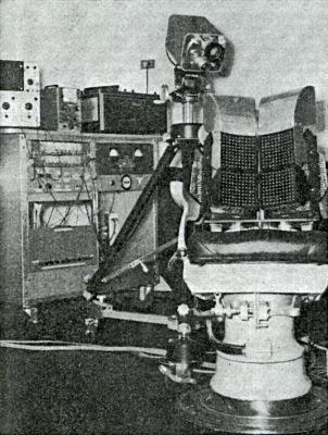
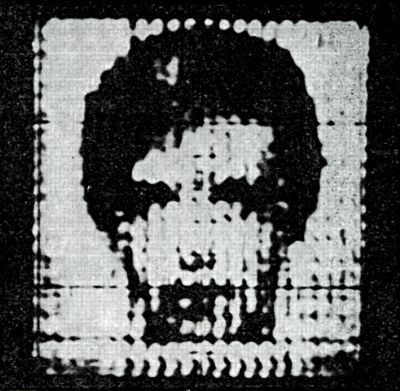
With the help of an oscilloscope it was possible to visualize the image created by the vibration of stimulants.
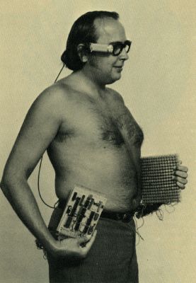
A year later, Paul developed a mobile version of his system:
1970s mobile visor
The man looks like Mavrodi, but this is not him.
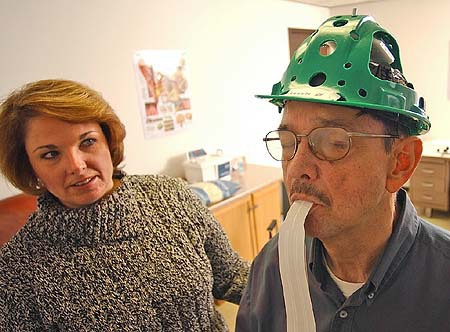
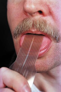
Nowadays, instead of tactile signal transmission, a “short” path is used through a more sensitive organ - the language. As they write in the articles, a few hours are enough to begin to perceive the image by the receptors of the tongue.
modern option
Think he eats noodles? But no, he looks with his tongue.
And it is not surprising that they are trying to monetize this discovery :
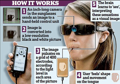
And it is not surprising that they are trying to monetize this discovery :
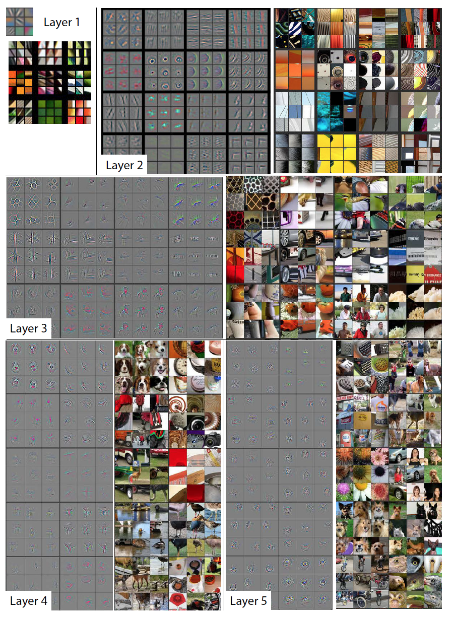
So how does it work? Speaking in simple language (not biologists and neurophysiologists, but rather in the language of data analysis), neurons are trained to efficiently extract features and draw conclusions on them. Replacing the usual signal with some other one , our neural network still extracts good low-level features (for example, computer vision, given below, these will be different gradient transitions or patterns) on layers that are located close to the sensor (eye, tongue, ear, etc.). d.). Deeper layers try to extract high-level signs (wheel, window). And probably, if we look for a wheel from a car in a sound signal, most likely we will not find it. Unfortunately, we will not be able to see which signs are extracted by neurons, but thanks to the article " Visualizing and Understanding Convolutional Networks " it is possible to look at the low-level and high-level signs extracted by the deep convolutional neural network. This, of course, is not a biological network, and perhaps everything is wrong in reality. At a minimum, it gives some kind of intuitive understanding of the reasons for seeing even the receptors of the tongue.
The large picture in the spoiler shows several features of each convolutional layer and parts of the original images that activate them. As you can see, the deeper, the less abstract the signs become.
Fully trained model
Each gray square corresponds to a visualization of the filter (which is used for convolution) or the weights of one neuron, and each color image is the part of the original image that activates the corresponding neuron. For clarity, neurons within a single layer are grouped into subject groups.
It can be assumed that, replacing the sensors, our brain does not need to completely retrain all neurons, it is enough to retrain only those that extract the high-level signs — and the rest are already able to extract quality features. Practice shows that this is approximately what it is. It is unlikely that in a couple of hours of walking with a plate in the tongue, the brain has time to remove and then grow new synaptic connections without losing the ability to feel the taste of food by the receptors of the tongue.
And now let's remember how the history of artificial neural networks began. In 1949, Donald Hebb publishes the book The Organization of Behavior , in which he describes the first principles of ANN training . It is worth noting that modern learning algorithms are not far from these principles.
- if nearby neurons are activated synchronously , the connection between them is enhanced ;
- if nearby neurons are activated asynchronously , the connection between them weakens (in fact, Hebb did not have this rule, he added it as an addition later).
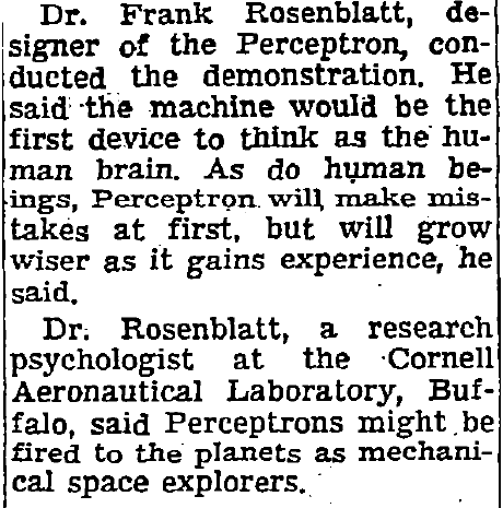
After nine years, Frank Rosenblatt creates the first model for teaching with a teacher, the perceptron . The author of the first artificial neural network did not pursue the goal of creating a universal approximator. He was a neurophysiologist, and his task was to create a device that could be trained like a human being. Just take a look at what journalists write about the perceptron. IMHO, this is charming:
New York Time, July 8, 1958
...
...
In perceptron, the Hebba learning rules were implemented. As we can see, synaptic plasticity in the rules has already been taken into account to some extent. And in principle, online learning gives us some plasticity - a neural network can constantly be trained on a continuous data stream, and its predictions in this regard will change over time, constantly taking into account changes in data. But there are no recommendations on other aspects of neuroplasticity, such as sensory replaceability or neurogenesis. But this is not surprising, just a little more than 20 years remain before the adoption of neuroplasticity. Given the subsequent history of ANN, the scientist was not in the mood for imitation of neuroplasticity, the question was about the survival rate of the theory in principle. Only after another renaissance of neural networks in the two thousand years, thanks to people like Hinton , LeKun , Bengio and Schmidthuber , other scientists had the opportunity to comprehensively approach machine learning and come to the concept of transfer learning.
Transfer learning
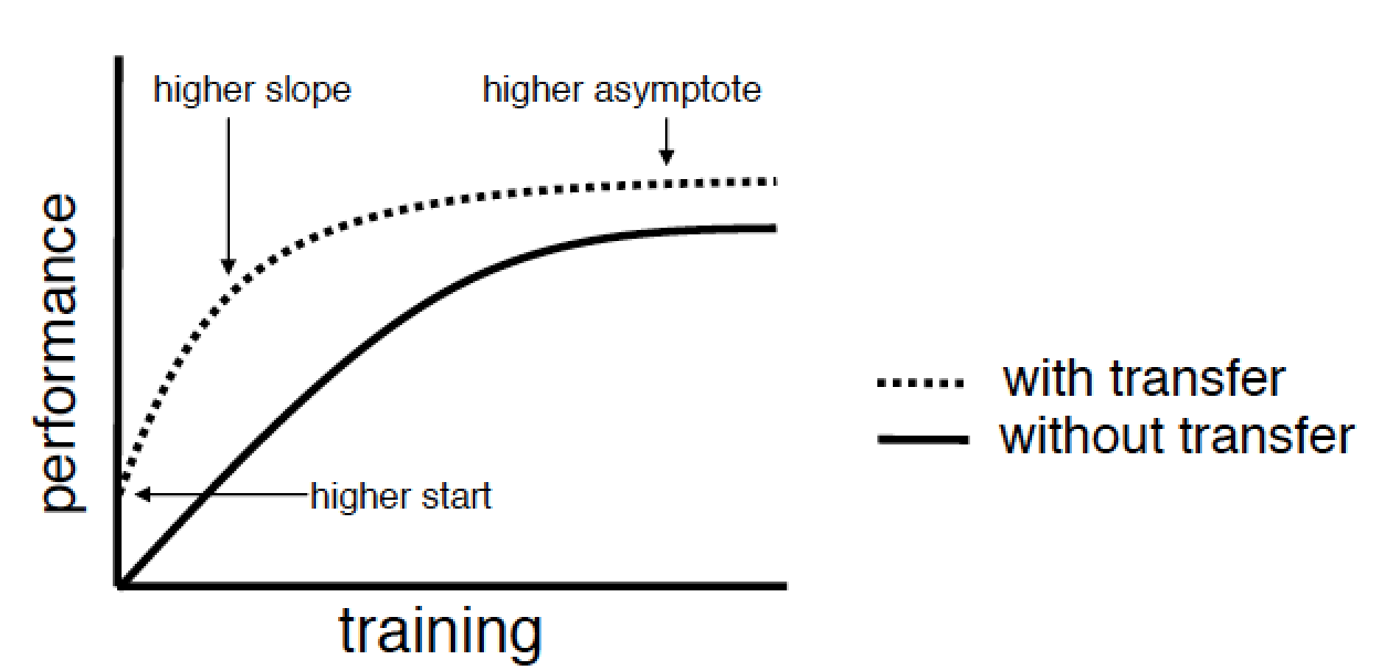
We define the goals of transfer learning. The authors of the publication of 2009 with the same name identify three main goals:
- higher start - improving the quality of education already at the initial iterations due to a more thorough selection of the initial parameters of the model or some other a priori information;
- higher slope - acceleration of the convergence of the learning algorithm;
- higher asymptote - improving the upper reachable quality boundary.
If you are familiar with the pre -training of deep networks with the help of auto-encoders or limited Boltzmann machines, then you will immediately think: “So this is, I already turned out to practice transfer learning or, at least, know how to do it.” But it turns out, no. The authors draw a clear distinction between standard machine learning and transfer learning. In the standard approach, you only have a goal and a data set, and the task is to achieve this goal by any means. As part of solving the problem, you can build a deep network, pre-train it with a greedy algorithm, build about a dozen of them and make an ensemble of them in some way. But all this will be within the framework of solving a single problem, and the time spent on solving such a problem will be comparable to the total time spent on training each model and its pre-training.
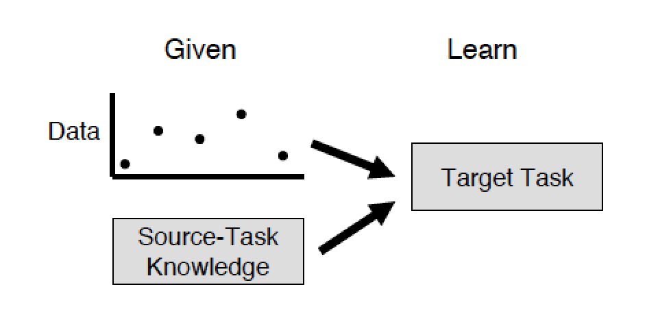
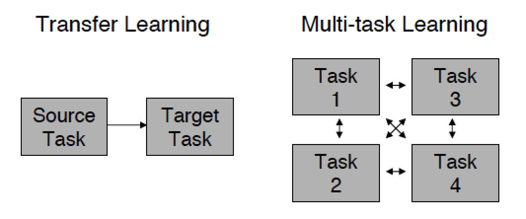
Now imagine that there are two tasks, and perhaps even different people have solved them. One of them uses part of the model of the other (source task) to reduce the time spent on creating a model from scratch and improve the performance of its model (target task). The process of transferring knowledge from one problem to another is transfer learning. And our brain probably does that. As in the example above, his real task is to feel the taste of the receptors of the tongue and see with his eyes. The challenge is to perceive the visual information by the receptors of the language. And instead of growing new neurons or losing weight of old ones and training them anew, the brain simply slightly adjusts the existing neural network to achieve the result.
Another feature of transfer learning is that information can only be transferred from the old model to the new one, because the old problem has long been solved. While with the standard approach, different models involved in solving a problem can exchange information with each other.
This post applies only to the part of transfer learning, which relates to the task of learning with a teacher, but I recommend interested readers to read the original. From there, you will learn that, say, in training with reinforcements or when training Bayesian networks, transfer learning was used earlier than in neural networks.
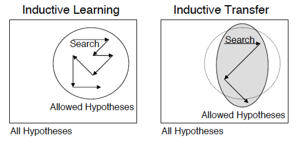
So, learning with a teacher is learning from labeled examples, while the learning process with examples is sometimes called inductive learning (transition from particular to general), and the generalizing ability is called inductive bias . Hence the second name of transfer learning - inductive transfer . Then we can say that the task of transferring knowledge in inductive learning is to allow the knowledge accumulated in the learning process of the old model to influence the generalizing ability of the new model (even when solving a different task).
Knowledge transfer can also be considered as some regularization, which limits the search space to a certain set of valid and good hypotheses.
Practice
I hope that by this time you are imbued with this, at first glance, unremarkable approach, as a transfer of knowledge. After all, you can simply say that no this is not a transfer of knowledge, neuroplasticity is far-fetched, and the best name for this method is copy-paste. Then you are just a pragmatist. This, of course, is also not bad, and then at least you will like the third section. Let's try to repeat something similar to that described in the first section, but on an artificial neural network.
First, we formulate the problem. Suppose you have a very large set of images. It is necessary to organize a search for similar images. This raises two problems. First, the measure of similarity between the images is not obvious, and if you just take the Euclidean distance from the n * m-dimensional vector, the result will not be very satisfactory. Secondly, even if there is a quality measure, it will not allow us to avoid a full scan of the base, and the base may contain billions of images.
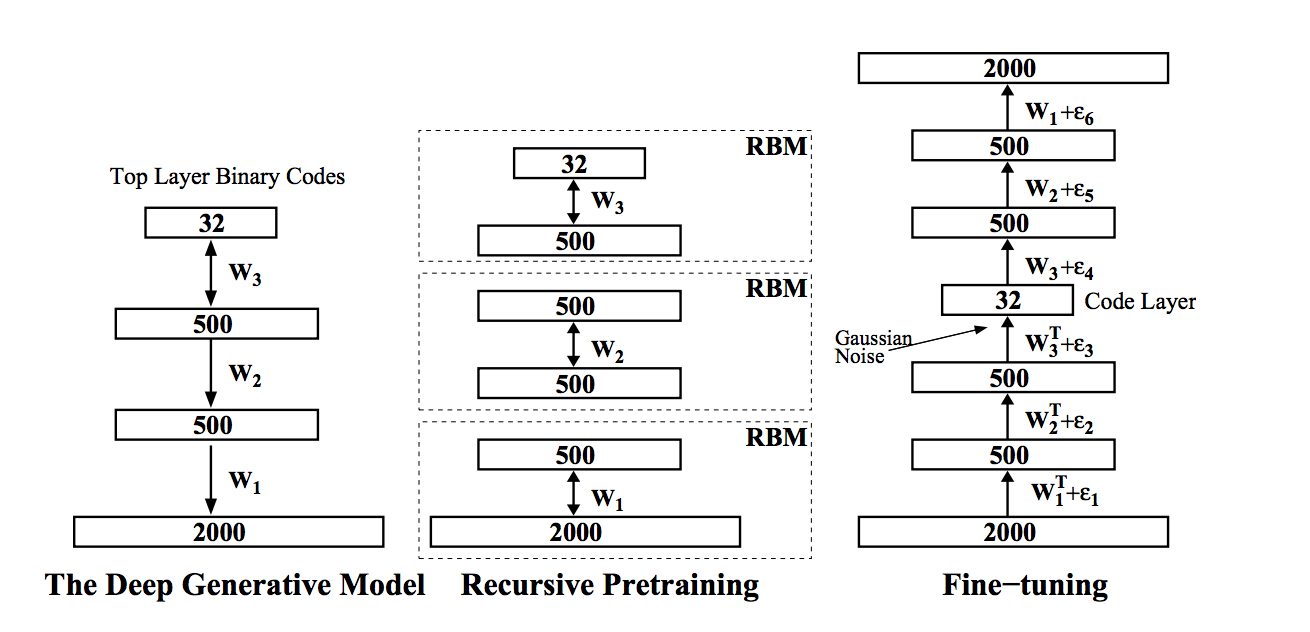
To solve this problem, you can use semantic hashing, one of these methods is described by Salakhudinov and Hinton in the article Semantic Hashing . Their idea is that the original data vector is encoded by a binary vector of small dimension (in our case, this is an image, and in the original article this is a binary vector of bag of words ). With this encoding, you can search for similar images for a linear time from the code length using the Hamming distance . Such encoding is called semantic, since images (texts, music, etc.) that are close in meaning and content in the new feature space are located close to each other. To implement this idea, they used a deep network of trust , the learning algorithm of which was developed by Hinton and the company back in 2006:
- the input network generally takes real values (gaussian-bernoulli rbm) and encodes them into a long binary vector, each next layer tries to reduce the length of the binary code (berboulli-bernoulli rbm);
- such a network is taught consistently from bottom to top by its own limited Boltzmann machine, where each next one uses the output of the previous one as its input data;
- then the network unfolds in the reverse order and learns as a deep auto-encoder , which receives a slightly noisy vector at the entrance, and it tries to restore the original, non-noisy image; this step is called fine turning;
- after all, the binary image in the middle of the auto-encoder will be the binary hash from the input image.
It seems to me that this is a brilliant model, and I decided that, in principle, the problem was solved, thanks to Hinton. I ran pre-training on the NVIDIA Tesla K20, waited a couple of days, and it turned out that everything is not as rosy as Hinton describes. Whether because the pictures are large, or because I used gaussian-bernoulli rbm, and the article uses poisson-bernoulli rbm, or because of the specificity of the data, and maybe, in general, I taught little . But I didn’t want to wait any longer. And then I remembered the advice of Maxim Milakov - use convolutional networks, as well as the term transfer learning from one of his presentations. There were, of course, other options, ranging from compressing the dimension of pictures and quantifying colors, to classic signs of computer vision and combining them into bags of visual words . But once I entered the deep learning path, it’s not so easy to wind up from it, and the bonuses that transfer learning promises (especially time savings) deceive me.
It turned out that the VGG group mentioned at the beginning, which won ImageNet competition in 2014, put its trained neural network into free access for non-commercial use , so I downloaded it purely for research purposes.
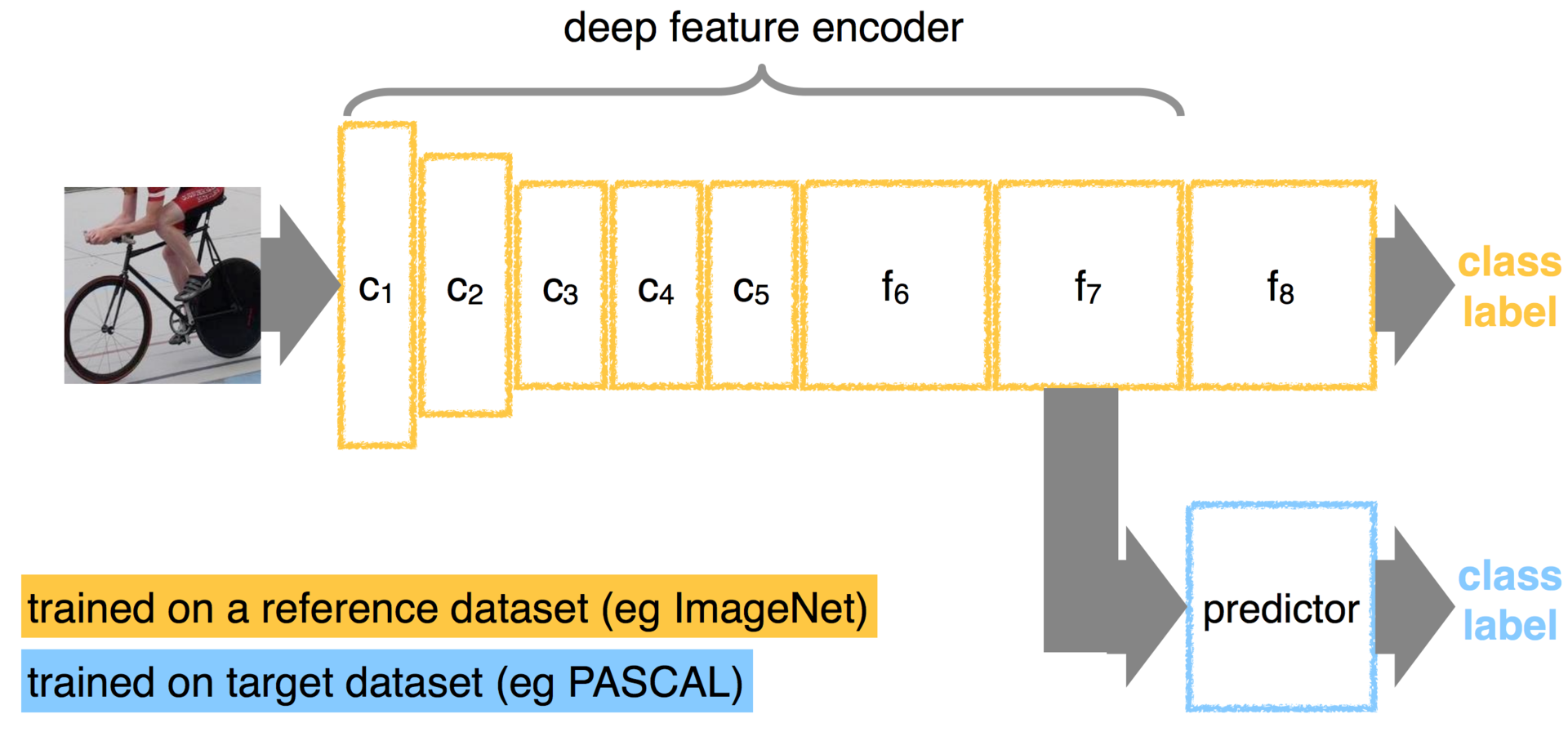
In general, ImageNet is not only a competition, but also a database of images, which contains a little more than one million real images. Each image is assigned to one of 1000 classes. The set is class-balanced, that is, just over 1000 images per class. The guys from Oxford won localization and classification in the nomination. Since there may be more than one objects in the images, the assessment is based on whether the correct answer is in the top 5 most likely options according to the model version. In the image below you can see an example of one of the models in the pictures from imagenet. Pay attention to the funny mistake with the Dalmatian, the model, unfortunately, did not find a cherry there.
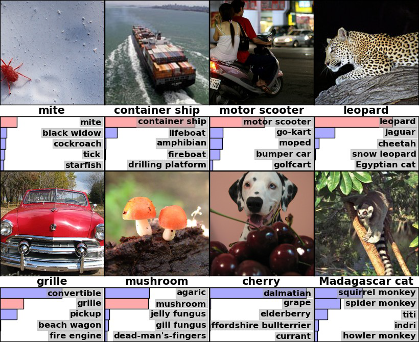
With such variability of dataset, it is logical to assume that somewhere in the network there is an effective feature extractor, as well as a classifier, which decides which class the image belongs to. I would like to get this very extractor, separate it from the classifier, and use it to teach deep autoencoder from the article on semantic hashing.
VGG neural network is trained and saved in Caffe format. Very cool library for deep learning, and most importantly - easy to learn, I recommend to read. Before trepanning the VGG network using caffe, I suggest to get a glimpse of the network itself. If the details are interesting, then I recommend the original article - Very Deep Convolutional Networks for Large-Scale Image Recognition (the name already hints at the depth of the network). And those who are not familiar with convolutional networks at all, you should at least read the Russian Wikipedia before moving on, it will not take more than 5-10 minutes (or there is a small description on Habré ).
So, for the article and the contest, the authors have trained several models:
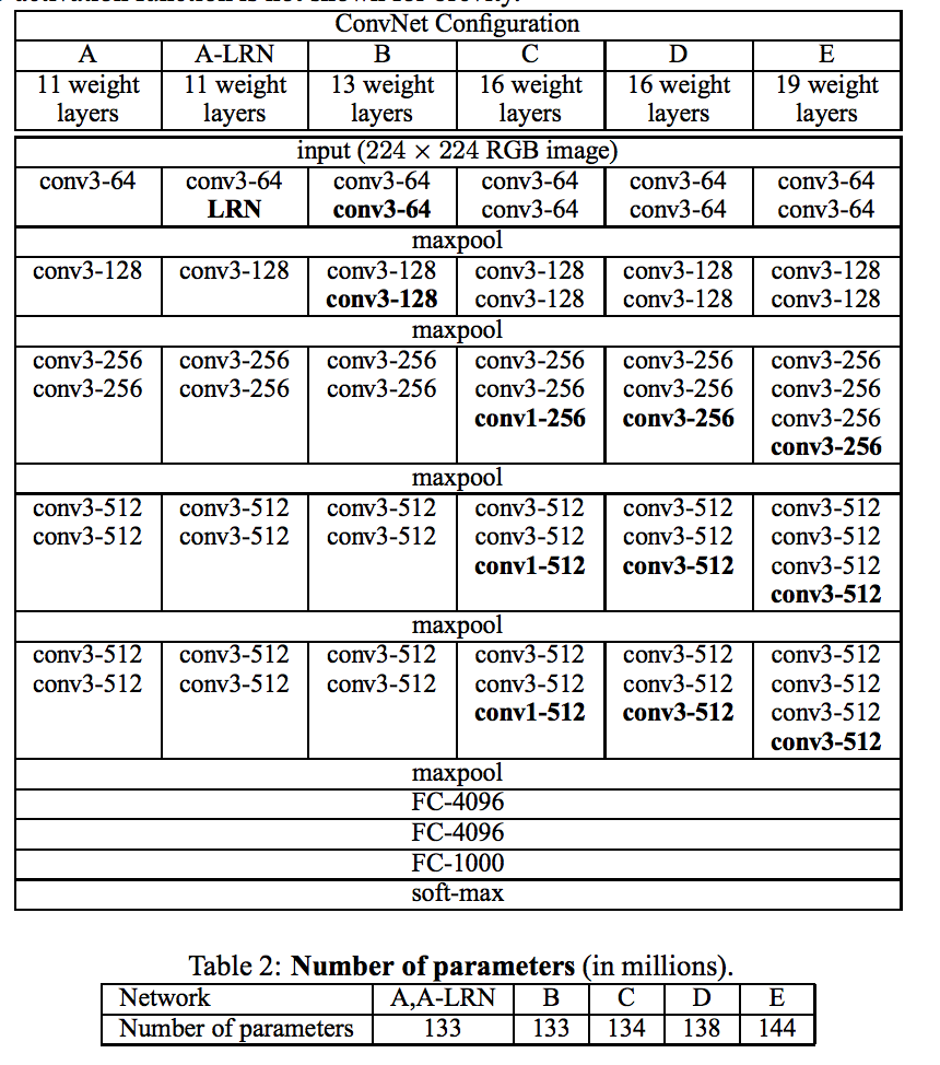
On their page they laid out the variants D and E. For the experiment we take the 19-layer variant E, in which the first 16 layers are convolutional, and the last three are fully connected. The last three layers are sensitive to the size of the images, so for the experiment, without thinking twice, I threw them out and left the first 16 layers, considering that I deleted the high-level features.
The caffe library uses the Google Protocol Buffers for model description, and the full description of the network is as follows.
19-layer model
name: "VGG_ILSVRC_19_layers" input: "data" input_dim: 10 input_dim: 3 input_dim: 224 input_dim: 224 layers { bottom: "data" top: "conv1_1" name: "conv1_1" type: CONVOLUTION convolution_param { num_output: 64 pad: 1 kernel_size: 3 } } layers { bottom: "conv1_1" top: "conv1_1" name: "relu1_1" type: RELU } layers { bottom: "conv1_1" top: "conv1_2" name: "conv1_2" type: CONVOLUTION convolution_param { num_output: 64 pad: 1 kernel_size: 3 } } layers { bottom: "conv1_2" top: "conv1_2" name: "relu1_2" type: RELU } layers { bottom: "conv1_2" top: "pool1" name: "pool1" type: POOLING pooling_param { pool: MAX kernel_size: 2 stride: 2 } } layers { bottom: "pool1" top: "conv2_1" name: "conv2_1" type: CONVOLUTION convolution_param { num_output: 128 pad: 1 kernel_size: 3 } } layers { bottom: "conv2_1" top: "conv2_1" name: "relu2_1" type: RELU } layers { bottom: "conv2_1" top: "conv2_2" name: "conv2_2" type: CONVOLUTION convolution_param { num_output: 128 pad: 1 kernel_size: 3 } } layers { bottom: "conv2_2" top: "conv2_2" name: "relu2_2" type: RELU } layers { bottom: "conv2_2" top: "pool2" name: "pool2" type: POOLING pooling_param { pool: MAX kernel_size: 2 stride: 2 } } layers { bottom: "pool2" top: "conv3_1" name: "conv3_1" type: CONVOLUTION convolution_param { num_output: 256 pad: 1 kernel_size: 3 } } layers { bottom: "conv3_1" top: "conv3_1" name: "relu3_1" type: RELU } layers { bottom: "conv3_1" top: "conv3_2" name: "conv3_2" type: CONVOLUTION convolution_param { num_output: 256 pad: 1 kernel_size: 3 } } layers { bottom: "conv3_2" top: "conv3_2" name: "relu3_2" type: RELU } layers { bottom: "conv3_2" top: "conv3_3" name: "conv3_3" type: CONVOLUTION convolution_param { num_output: 256 pad: 1 kernel_size: 3 } } layers { bottom: "conv3_3" top: "conv3_3" name: "relu3_3" type: RELU } layers { bottom: "conv3_3" top: "conv3_4" name: "conv3_4" type: CONVOLUTION convolution_param { num_output: 256 pad: 1 kernel_size: 3 } } layers { bottom: "conv3_4" top: "conv3_4" name: "relu3_4" type: RELU } layers { bottom: "conv3_4" top: "pool3" name: "pool3" type: POOLING pooling_param { pool: MAX kernel_size: 2 stride: 2 } } layers { bottom: "pool3" top: "conv4_1" name: "conv4_1" type: CONVOLUTION convolution_param { num_output: 512 pad: 1 kernel_size: 3 } } layers { bottom: "conv4_1" top: "conv4_1" name: "relu4_1" type: RELU } layers { bottom: "conv4_1" top: "conv4_2" name: "conv4_2" type: CONVOLUTION convolution_param { num_output: 512 pad: 1 kernel_size: 3 } } layers { bottom: "conv4_2" top: "conv4_2" name: "relu4_2" type: RELU } layers { bottom: "conv4_2" top: "conv4_3" name: "conv4_3" type: CONVOLUTION convolution_param { num_output: 512 pad: 1 kernel_size: 3 } } layers { bottom: "conv4_3" top: "conv4_3" name: "relu4_3" type: RELU } layers { bottom: "conv4_3" top: "conv4_4" name: "conv4_4" type: CONVOLUTION convolution_param { num_output: 512 pad: 1 kernel_size: 3 } } layers { bottom: "conv4_4" top: "conv4_4" name: "relu4_4" type: RELU } layers { bottom: "conv4_4" top: "pool4" name: "pool4" type: POOLING pooling_param { pool: MAX kernel_size: 2 stride: 2 } } layers { bottom: "pool4" top: "conv5_1" name: "conv5_1" type: CONVOLUTION convolution_param { num_output: 512 pad: 1 kernel_size: 3 } } layers { bottom: "conv5_1" top: "conv5_1" name: "relu5_1" type: RELU } layers { bottom: "conv5_1" top: "conv5_2" name: "conv5_2" type: CONVOLUTION convolution_param { num_output: 512 pad: 1 kernel_size: 3 } } layers { bottom: "conv5_2" top: "conv5_2" name: "relu5_2" type: RELU } layers { bottom: "conv5_2" top: "conv5_3" name: "conv5_3" type: CONVOLUTION convolution_param { num_output: 512 pad: 1 kernel_size: 3 } } layers { bottom: "conv5_3" top: "conv5_3" name: "relu5_3" type: RELU } layers { bottom: "conv5_3" top: "conv5_4" name: "conv5_4" type: CONVOLUTION convolution_param { num_output: 512 pad: 1 kernel_size: 3 } } layers { bottom: "conv5_4" top: "conv5_4" name: "relu5_4" type: RELU } layers { bottom: "conv5_4" top: "pool5" name: "pool5" type: POOLING pooling_param { pool: MAX kernel_size: 2 stride: 2 } } layers { bottom: "pool5" top: "fc6" name: "fc6" type: INNER_PRODUCT inner_product_param { num_output: 4096 } } layers { bottom: "fc6" top: "fc6" name: "relu6" type: RELU } layers { bottom: "fc6" top: "fc6" name: "drop6" type: DROPOUT dropout_param { dropout_ratio: 0.5 } } layers { bottom: "fc6" top: "fc7" name: "fc7" type: INNER_PRODUCT inner_product_param { num_output: 4096 } } layers { bottom: "fc7" top: "fc7" name: "relu7" type: RELU } layers { bottom: "fc7" top: "fc7" name: "drop7" type: DROPOUT dropout_param { dropout_ratio: 0.5 } } layers { bottom: "fc7" top: "fc8" name: "fc8" type: INNER_PRODUCT inner_product_param { num_output: 1000 } } layers { bottom: "fc8" top: "prob" name: "prob" type: SOFTMAX } In order to make the described trepanation, it is enough to delete all layers in the model description, starting from fc6 (full connected layer). But it is worth noting that then the output of the network will be unlimited from above, since The activation function is the rectified linear unit :
Such a question is conveniently solved by taking a sigmoid from the network output. We can hope that many neurons will either be 0 or some large number. Then after taking the sigmoid, we get a lot of units and 0.5 (sigmoid from 0 is 0.5). If we normalize the obtained values in the interval from 0 to 1, then they can be interpreted as the probabilities of activation of neurons, and almost all of them will be in the region of zero or one. The probability of activation of a neuron is interpreted as the probability of the presence of a trait in the image (for example, is there a human eye on it).
Here is the typical answer of such a network in my case:
normalized sigmoid from the last convolutional layer
0.0
0.0
0.0
0.0
0.0
0.0
1.0
0.0
0.0
0.0
0.0
0.0
0.0
0.0
0.0
0.0
0.0
0.0
0.0
0.0
0.0
0.0
0.0
0.0
0.0
0.0
0.0
0.0
0.0
0.0
0.0
0.0
0.0
0.0
0.0
0.0
0.994934
0.0
0.0
0.999047
0.829219
0.0
0.0
0.0
0.0
0.0
0.0
0.0
0.0
0.0
0.0
0.0
0.997255
0.0
0.0
0.0
0.0
0.0
0.0
0.0
1.0
1.0
0.0
0.999382
0.0
0.0
0.0
0.0
0.988762
0.0
0.0
1.0
1.0
0.0
1.0
1.0
0.0
1.0
1.0
1.0
1.0
1.0
0.0
1.0
1.0
0.0
0.0
1.0
1.0
0.0
1.0
1.0
0.0
0.0
0.0
0.0
0.0
0.847886
0.0
0.0
0.0
0.0
0.957379
0.0
0.0
0.0
0.0
0.0
1.0
0.999998
0.0
0.0
0.0
0.0
0.0
0.0
0.0
0.0
0.0
0.0
0.0
0.0
0.0
0.0
0.0
0.0
1.0
0.999999
0.0
0.54814
0.739735
0.0
0.0
0.0
0.912179
0.0
0.0
0.78984
0.0
0.0
0.0
0.0
0.0
0.0
0.0
0.681776
0.0
0.0
0.991501
0.0
0.999999
0.999152
0.0
0.0
1.0
0.0
0.0
0.0
0.0
0.999996
1.0
0.0
1.0
1.0
0.0
0.880588
0.0
0.0
0.0
0.0
0.0
0.0
0.836756
0.995515
0.0
0.999354
0.0
1.0
1.0
0.0
1.0
1.0
0.0
0.999897
0.0
0.953126
0.0
0.0
0.999857
0.0
0.0
0.937695
0.999983
1.0
0.0
0.0
0.0
0.0
0.0
1.0
0.0
0.0
0.0
0.0
0.0
0.0
0.0
0.0
1.0
0.0
0.0
0.0
0.0
0.0
0.0
0.0
0.0
0.0
0.0
0.0
0.0
0.0
0.0
0.0
0.0
0.0
0.0
0.0
0.0
0.0
0.0
0.0
0.0
0.0
0.0
0.0
0.0
0.0
0.994934
0.0
0.0
0.999047
0.829219
0.0
0.0
0.0
0.0
0.0
0.0
0.0
0.0
0.0
0.0
0.0
0.997255
0.0
0.0
0.0
0.0
0.0
0.0
0.0
1.0
1.0
0.0
0.999382
0.0
0.0
0.0
0.0
0.988762
0.0
0.0
1.0
1.0
0.0
1.0
1.0
0.0
1.0
1.0
1.0
1.0
1.0
0.0
1.0
1.0
0.0
0.0
1.0
1.0
0.0
1.0
1.0
0.0
0.0
0.0
0.0
0.0
0.847886
0.0
0.0
0.0
0.0
0.957379
0.0
0.0
0.0
0.0
0.0
1.0
0.999998
0.0
0.0
0.0
0.0
0.0
0.0
0.0
0.0
0.0
0.0
0.0
0.0
0.0
0.0
0.0
0.0
1.0
0.999999
0.0
0.54814
0.739735
0.0
0.0
0.0
0.912179
0.0
0.0
0.78984
0.0
0.0
0.0
0.0
0.0
0.0
0.0
0.681776
0.0
0.0
0.991501
0.0
0.999999
0.999152
0.0
0.0
1.0
0.0
0.0
0.0
0.0
0.999996
1.0
0.0
1.0
1.0
0.0
0.880588
0.0
0.0
0.0
0.0
0.0
0.0
0.836756
0.995515
0.0
0.999354
0.0
1.0
1.0
0.0
1.0
1.0
0.0
0.999897
0.0
0.953126
0.0
0.0
0.999857
0.0
0.0
0.937695
0.999983
1.0
0.0
0.0
0.0
0.0
0.0
1.0
0.0
0.0
0.0
In caffe, this question is resolved as follows:
layers { bottom: "pool5" top: "sigmoid1" name: "sigmoid1" type: SIGMOID } In caffe, a python wrapper is implemented, and the following code initializes the network and makes normalization:
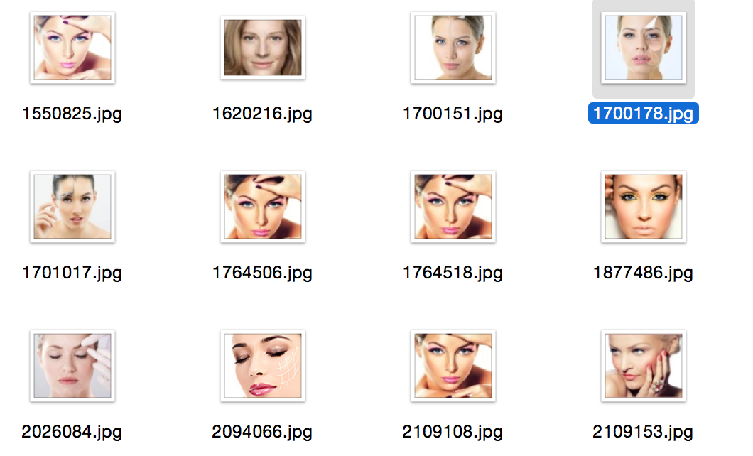
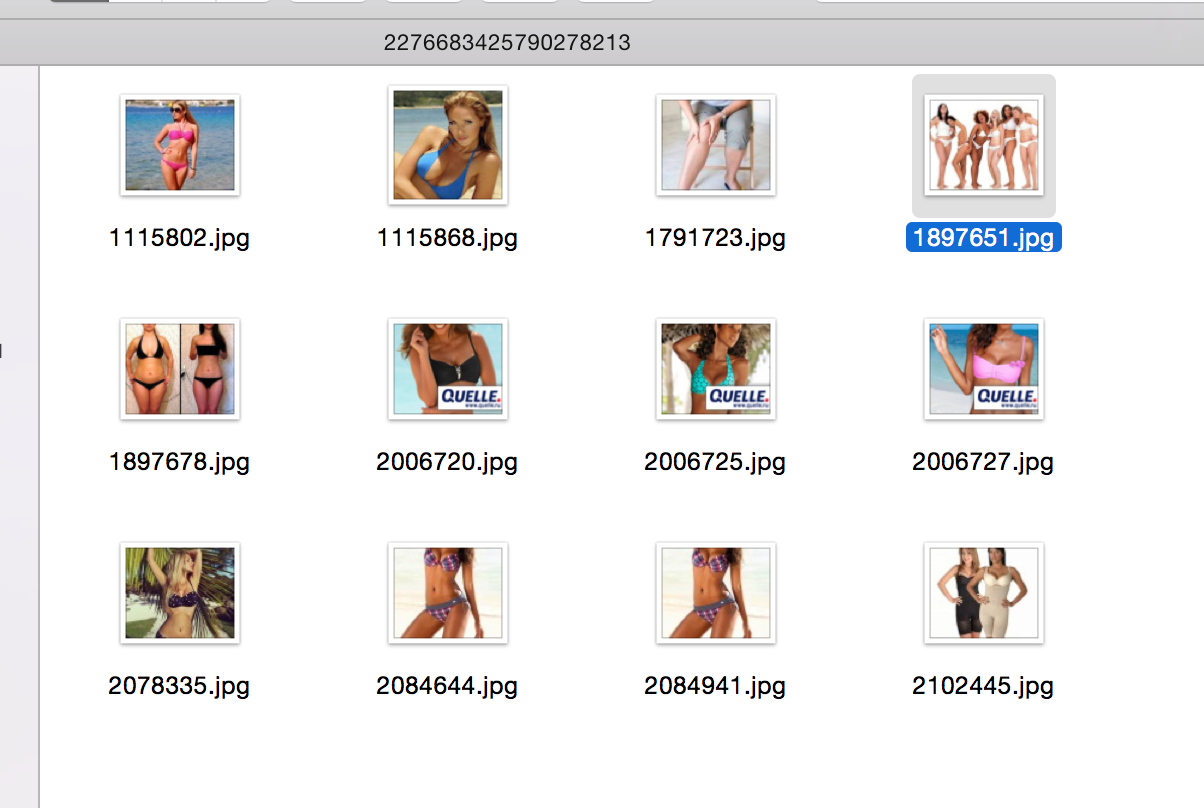
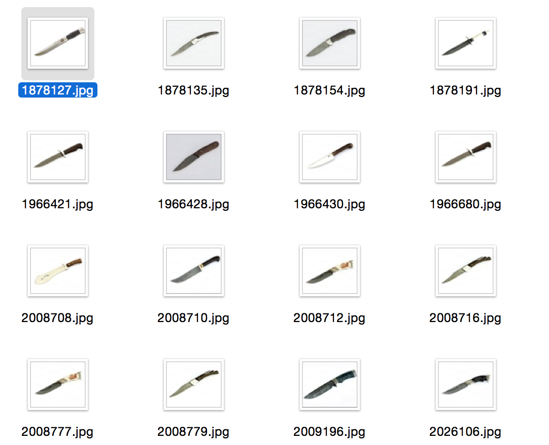
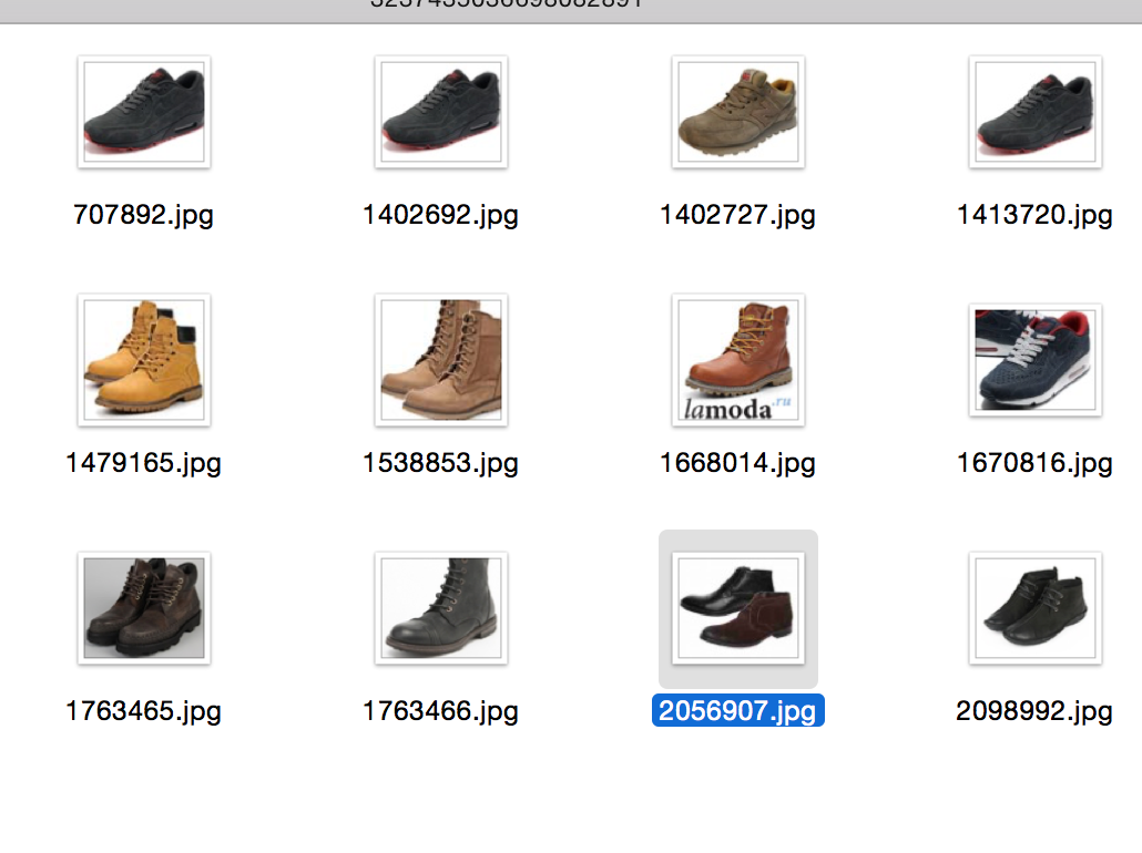
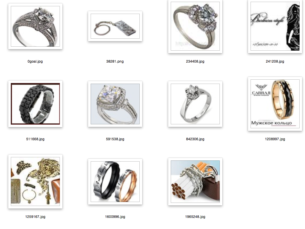
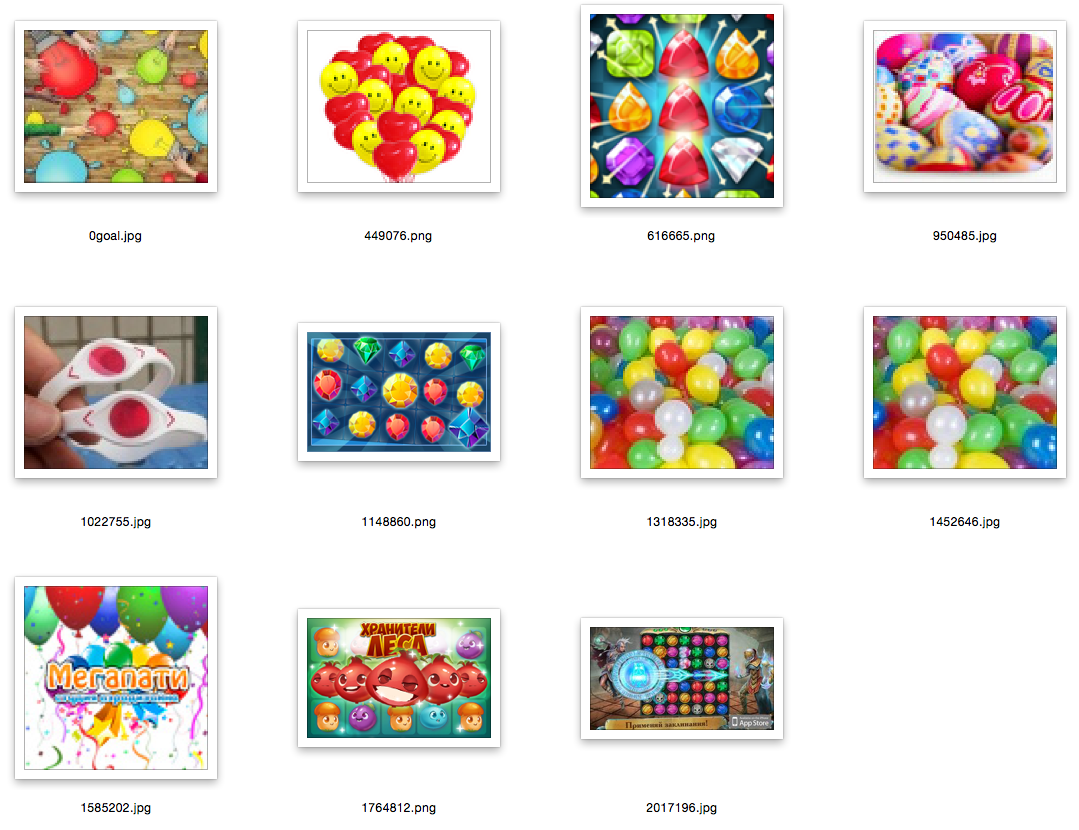
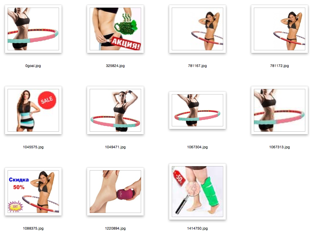
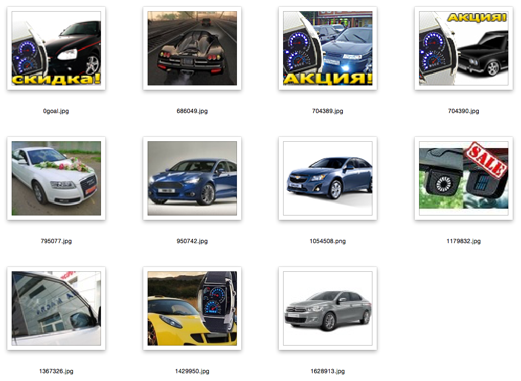
caffe.set_mode_gpu() net = caffe.Classifier('deploy.prototxt', 'VGG_ILSVRC_19_layers.caffemodel', channel_swap=(2,1,0), raw_scale=255, image_dims=(options.width, options.height)) #.................. out = net.forward_all(**{net.inputs[0]: caffe_in}) out = out['sigmoid1'].reshape(out['sigmoid1'].shape[0], np.prod(out['sigmoid1'].shape[1:])) out = (out - 0.5)/0.5 So, at the moment we have a binary (well or almost) representation of images with high-dimensional vectors, in my case 4608, it remains to train the Deep Befief Network to compress these representations. The resulting model has become an even deeper network. Without waiting for DBN to study for a few days, let's conduct an experiment to search: we will choose a random image and look for the next image for it, in terms of the Hamming distance. Notice, this is all on raw features, on a vector of high dimension, without any weighting of signs.
Explanations: The first picture is a picture request, a random image from the database; the rest are closest to her.
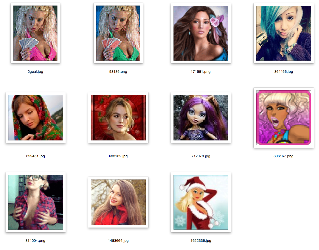
other examples in the spoiler


Conclusion and links
I think you can easily come up with an example in which you will not just transfer static layers, but also train them in your own way. Let's say you can initialize part of your network using another network and then retrain in your classes.
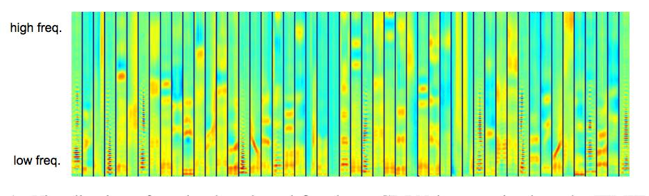
And if you try something closer to the experiment described in the first part? Please: Here is an example of an article using convolutional deep belief networks to extract features from audio signals. Why not use trained convolutions to initialize cDBN weights? What is such a spectrogram not an image, and why should low-level features not work on it:
If you want to experiment with the processing of natural language and try transfer learning, then here is a suitable article for LeKun to start. And yes, there, too, the text appears as an image.
In general, transfer learning is a great thing, and caffe is a cool library for deep learning.
There are a lot of links in the text, here are some of them:
- Tongue Vision
- Self-taught Learning: Transfer Learning from Unlabeled Data
- Transfer learning
- Large Scale Visual Recognition Challenge 2014 (ILSVRC2014)
- electricity for eyes
- Visualizing and Understanding Convolutional Networks
- Stacked Denoising Autoencoders: Learning Useful Representations in the Deep Network with a Local Denoising Criterion
- Semantic hashing
- Visual geometry group
- Very Deep Convolutional Networks for Large-Scale Visual Recognition (model)
- Caffe
- Very Deep Convolutional Networks for Large-Scale Visual Recognition (article)
- Image representations for large-scale visual recognition (A. Vedaldi from VGG)
Source: https://habr.com/ru/post/252965/
All Articles