Sound prints: radio advertising recognition
From this article, you will learn that recognizing even short sound fragments in a noisy recording is a completely solvable problem, and the prototype is generally implemented in 30 lines of Python code. We will see how the Fourier transform helps here, and we’ll see how the search and matching algorithm works. The article will be useful if you yourself want to write a similar system, or you wonder how it can be arranged.
To begin with, let us ask ourselves the question: who generally needs to recognize advertising on the radio? This is useful for advertisers who can track the real outputs of their commercials, catch cases of cropping or interruption; radio stations can monitor the output of network advertising in the regions, etc. The same problem of recognition arises if we want to track the playback of a piece of music (which the copyright holders are very fond of), or learn a song from a small fragment (as Shazam and other similar services do).
More strictly, the task is formulated as follows: we have a certain set of reference audio fragments (songs or commercials), and there is an audio recording of the air in which some of these fragments presumably sound. The task is to find all the fragments sounded, to determine the moments of the beginning and the duration of playback. If we analyze the recordings of the ether, then we need the system as a whole to work faster than real time.
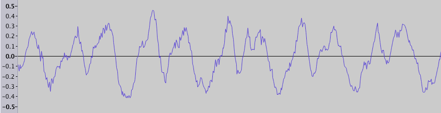
Everyone knows that sound (in the narrow sense) is a wave of compression and rarefaction, spreading through the air. Sound recording, for example in a wav file, is a sequence of amplitude values (physically, it corresponds to the degree of compression, or pressure). If you opened the audio editor, you probably saw the visualization of this data - a graph of the amplitude versus time (the fragment duration is 0.025 s):
')
But we do not perceive these fluctuations in frequency directly, but hear sounds of different frequencies and timbres. Therefore, another method of sound visualization is often used - the spectrogram , where time is represented on the horizontal axis, frequency is on the vertical axis, and the color of the point denotes amplitude. For example, here is a spectrogram of the sound of a violin, spanning several seconds in time:
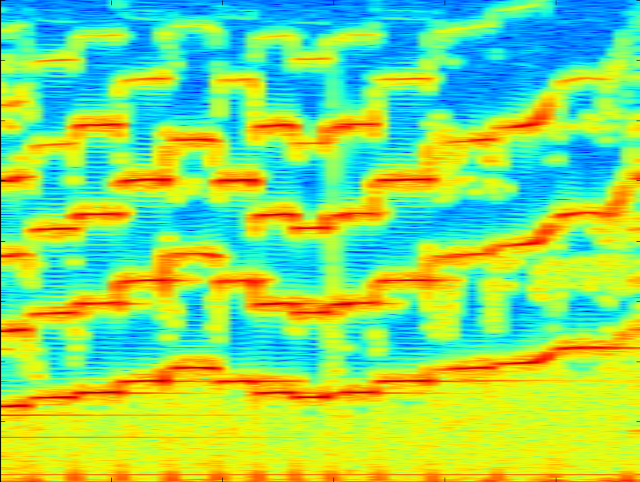
On it are visible individual notes and their harmonics, as well as noise - vertical stripes, covering the entire range of frequencies.
The task of searching for a fragment on the air can be divided into two parts: first, candidates are found among a large number of reference fragments, and then to check whether the candidate really sounds in this fragment of the ether, and if so, at what point the sound begins and ends. Both operations use for their work the “imprint” of a fragment of the sound. It must be noise resistant and compact enough. This imprint is constructed as follows: we divide the spectrogram into short segments of time, and in each such segment we search for a frequency with a maximum amplitude (in fact, it is better to look for several maxima in different ranges, but for simplicity we take one maximum in the most meaningful range). A set of such frequencies (or frequency indices) is an imprint. Very roughly, we can say that these are “notes” that sound at each moment in time.
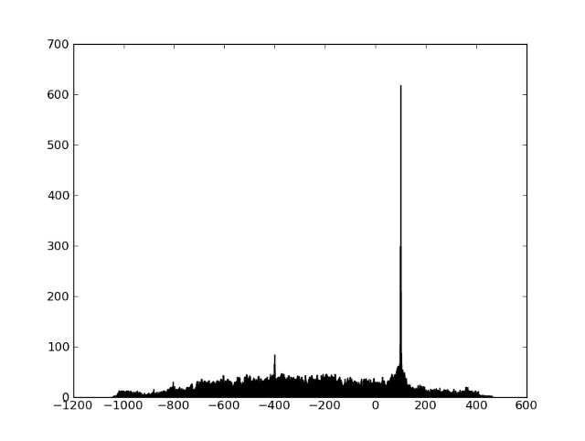
We can get an imprint of a fragment of the ether and all the reference fragments, and we will only have to learn how to quickly search for candidates and compare the fragments. First, look at the comparison task. It is clear that prints will never match exactly due to noise and distortion. But it turns out that the frequencies thus coarsened in such a way quite well survive all the distortions (the frequencies almost never “float”), and a sufficiently large percentage of frequencies coincide exactly - thus, we can only find a shift in which there are many coincidences among the two sequences of frequencies. A simple way to visualize this is to first find all the pairs of points that match in frequency, and then build a histogram of the time differences between the matching points. If two fragments have a common area, then there will be a pronounced peak on the histogram (and the peak position indicates the start time of the matched fragment):
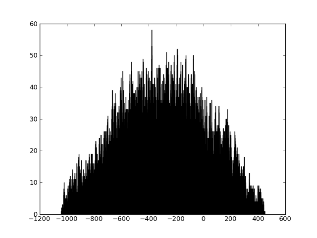
If the two fragments are not connected in any way, then there will be no peak:
The problem of finding candidates is usually solved with the use of hashing - a larger number of hashes is constructed from the fragment fingerprint, as a rule, these are several values from the fingerprint, reaching in a row or at some distance. Various approaches can be viewed at the links at the end of the article. In our case, the number of reference fragments was about a hundred, and it was possible to do without the candidate selection stage altogether.
On those records that we had, the F-score was 98.5%, and the accuracy of determining the beginning was about 1 s. As expected, most of the errors were on short (4-5 s) videos. But the main conclusion for me personally is that in such tasks a solution written independently often works better than a ready-made one (for example, from EchoPrint, about which they already wrote on Habré, it turned out to squeeze no more than 50-70% because of short clips) simply because that all tasks and data have their own specifics, and when there are many variations in the algorithm and a great deal of arbitrariness in the choice of parameters, understanding of all stages of work and visualization on real data greatly contributes to a good result.
Fun facts:
Literature:
To begin with, let us ask ourselves the question: who generally needs to recognize advertising on the radio? This is useful for advertisers who can track the real outputs of their commercials, catch cases of cropping or interruption; radio stations can monitor the output of network advertising in the regions, etc. The same problem of recognition arises if we want to track the playback of a piece of music (which the copyright holders are very fond of), or learn a song from a small fragment (as Shazam and other similar services do).
More strictly, the task is formulated as follows: we have a certain set of reference audio fragments (songs or commercials), and there is an audio recording of the air in which some of these fragments presumably sound. The task is to find all the fragments sounded, to determine the moments of the beginning and the duration of playback. If we analyze the recordings of the ether, then we need the system as a whole to work faster than real time.
How it works
Everyone knows that sound (in the narrow sense) is a wave of compression and rarefaction, spreading through the air. Sound recording, for example in a wav file, is a sequence of amplitude values (physically, it corresponds to the degree of compression, or pressure). If you opened the audio editor, you probably saw the visualization of this data - a graph of the amplitude versus time (the fragment duration is 0.025 s):
')
But we do not perceive these fluctuations in frequency directly, but hear sounds of different frequencies and timbres. Therefore, another method of sound visualization is often used - the spectrogram , where time is represented on the horizontal axis, frequency is on the vertical axis, and the color of the point denotes amplitude. For example, here is a spectrogram of the sound of a violin, spanning several seconds in time:
On it are visible individual notes and their harmonics, as well as noise - vertical stripes, covering the entire range of frequencies.
To build such a spectrogram using Python, you can:
You can use the SciPy library to load data from a wav file, and use matplotlib to build a spectrogram. All examples are given for Python version 2.7, but probably should work for version 3 as well. Suppose that file.wav contains a sound recording with a sampling frequency of 8000 Hz:
import numpy from matplotlib import pyplot, mlab import scipy.io.wavfile from collections import defaultdict SAMPLE_RATE = 8000 # Hz WINDOW_SIZE = 2048 # , fft WINDOW_STEP = 512 # def get_wave_data(wave_filename): sample_rate, wave_data = scipy.io.wavfile.read(wave_filename) assert sample_rate == SAMPLE_RATE, sample_rate if isinstance(wave_data[0], numpy.ndarray): # wave_data = wave_data.mean(1) return wave_data def show_specgram(wave_data): fig = pyplot.figure() ax = fig.add_axes((0.1, 0.1, 0.8, 0.8)) ax.specgram(wave_data, NFFT=WINDOW_SIZE, noverlap=WINDOW_SIZE - WINDOW_STEP, Fs=SAMPLE_RATE) pyplot.show() wave_data = get_wave_data('file.wav') show_specgram(wave_data) The task of searching for a fragment on the air can be divided into two parts: first, candidates are found among a large number of reference fragments, and then to check whether the candidate really sounds in this fragment of the ether, and if so, at what point the sound begins and ends. Both operations use for their work the “imprint” of a fragment of the sound. It must be noise resistant and compact enough. This imprint is constructed as follows: we divide the spectrogram into short segments of time, and in each such segment we search for a frequency with a maximum amplitude (in fact, it is better to look for several maxima in different ranges, but for simplicity we take one maximum in the most meaningful range). A set of such frequencies (or frequency indices) is an imprint. Very roughly, we can say that these are “notes” that sound at each moment in time.
Here's how to get a sound track print.
def get_fingerprint(wave_data): # pxx[freq_idx][t] - pxx, _, _ = mlab.specgram(wave_data, NFFT=WINDOW_SIZE, noverlap=WINDOW_OVERLAP, Fs=SAMPLE_RATE) band = pxx[15:250] # 60 1000 Hz return numpy.argmax(band.transpose(), 1) # max print get_fingerprint(wave_data) We can get an imprint of a fragment of the ether and all the reference fragments, and we will only have to learn how to quickly search for candidates and compare the fragments. First, look at the comparison task. It is clear that prints will never match exactly due to noise and distortion. But it turns out that the frequencies thus coarsened in such a way quite well survive all the distortions (the frequencies almost never “float”), and a sufficiently large percentage of frequencies coincide exactly - thus, we can only find a shift in which there are many coincidences among the two sequences of frequencies. A simple way to visualize this is to first find all the pairs of points that match in frequency, and then build a histogram of the time differences between the matching points. If two fragments have a common area, then there will be a pronounced peak on the histogram (and the peak position indicates the start time of the matched fragment):
If the two fragments are not connected in any way, then there will be no peak:
You can build such a wonderful histogram like this:
The files on which you can practice your recognition are here .
def compare_fingerprints(base_fp, fp): base_fp_hash = defaultdict(list) for time_index, freq_index in enumerate(base_fp): base_fp_hash[freq_index].append(time_index) matches = [t - time_index # for time_index, freq_index in enumerate(fp) for t in base_fp_hash[freq_index]] pyplot.clf() pyplot.hist(matches, 1000) pyplot.show() The files on which you can practice your recognition are here .
The problem of finding candidates is usually solved with the use of hashing - a larger number of hashes is constructed from the fragment fingerprint, as a rule, these are several values from the fingerprint, reaching in a row or at some distance. Various approaches can be viewed at the links at the end of the article. In our case, the number of reference fragments was about a hundred, and it was possible to do without the candidate selection stage altogether.
results
On those records that we had, the F-score was 98.5%, and the accuracy of determining the beginning was about 1 s. As expected, most of the errors were on short (4-5 s) videos. But the main conclusion for me personally is that in such tasks a solution written independently often works better than a ready-made one (for example, from EchoPrint, about which they already wrote on Habré, it turned out to squeeze no more than 50-70% because of short clips) simply because that all tasks and data have their own specifics, and when there are many variations in the algorithm and a great deal of arbitrariness in the choice of parameters, understanding of all stages of work and visualization on real data greatly contributes to a good result.
Fun facts:
- On the spectrogram of one of the tracks of the Aphex Twin group there is a human face
- The author of the article, which reproduced the Shazam algorithm in Java, received threats from their lawyers
Literature:
Source: https://habr.com/ru/post/252937/
All Articles