Perspective matrices in graphic API or the devil hides in details
At a certain point, any developer in the field of computer graphics raises the question: how do these advanced matrices work? Sometimes the answer is very difficult to find and, as is usually the case, the majority of developers throw this activity halfway through.
This is not a solution! Let's figure it out together!
Let's be realistic with a practical bias and take as an experimental OpenGL version 3.3. Starting with this version, each developer is obliged to independently implement the module of matrix operations. Great, this is what we need. Let's decompose ours with you a difficult task and highlight the main points. Some facts from the OpenGL specification:
There are two ways to store matrices: cool-major and row-major. In lectures on linear algebra, the row-major scheme is used. By and large, the representation of matrices in memory does not matter, because the matrix can always be translated into one type of representation into another by simple transposition. And if there is no difference, then for all subsequent calculations we will use the classic row-major matrices. When programming OpenGL, there is a small trick that allows you to abandon the transposition of matrices while maintaining the classic row-major calculations. In the shader program, the matrix needs to be transferred as it is, and in the shader it is necessary to multiply not the vector by the matrix, but the matrix by the vector.
')
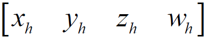
Homogeneous coordinates is not a very tricky system with a number of simple rules for translating the usual Cartesian coordinates into homogeneous coordinates and back. The uniform coordinate is a [1x4] dimension row matrix. In order to translate the Cartesian coordinate into a homogeneous coordinate, x , y and z must be multiplied by any real number w (except 0). Next, you need to write the result in the first three components, and the last component will be equal to the factor w . In other words:
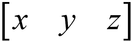 - Cartesian coordinates
w is a real number not equal to 0
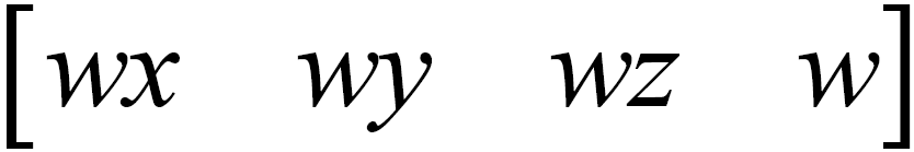 - homogeneous coordinates
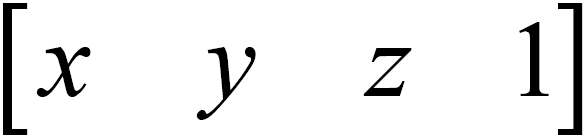
A little trick: If w is equal to one, then all that is needed for translation is to transfer the components x , y and z and assign the unit to the last component. That is, get the matrix row:
A few words about zero as w . From the point of view of homogeneous coordinates, this is quite permissible. Homogeneous coordinates allow you to distinguish points and vectors. In the Cartesian coordinate system, such a separation is impossible.
- point where ( x, y, z ) - Cartesian coordinates
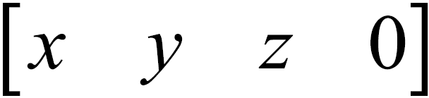 Is a vector, where ( x, y, z ) is a radius vector
The reverse translation of a vertex from homogeneous coordinates to Cartesian coordinates is carried out as follows. All components of the matrix-row must be divided into the last component. In other words:
 - homogeneous coordinates
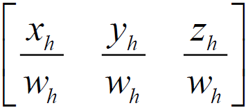 - Cartesian coordinates
The main thing that you need to know is that all OpenGL algorithms for clipping and rasterization work in Cartesian coordinates, but before that, all the transformations are performed in homogeneous coordinates. The transition from homogeneous coordinates to Cartesian coordinates is carried out by hardware.
The canonical clipping volume or Canonic view volume (CVV) is one of the less documented parts of OpenGL. As can be seen from fig. 1 CVV is a cube aligned along the axes with the center at the origin and the edge length equal to two. Anything that enters the CVV area is subject to rasterization; anything outside the CVV is ignored. Anything that partially goes beyond CVV boundaries is subject to clipping algorithms. The most important thing to know is the CVV coordinate system is left-sided!
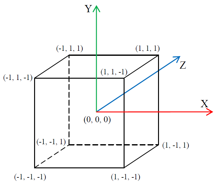
Fig. 1. OpenGL canonical clipping volume (CVV)
Left side coordinate system? How so, because in the OpenGL 1.0 specification it is clearly written that the coordinate system used is right-handed? Let's figure it out.
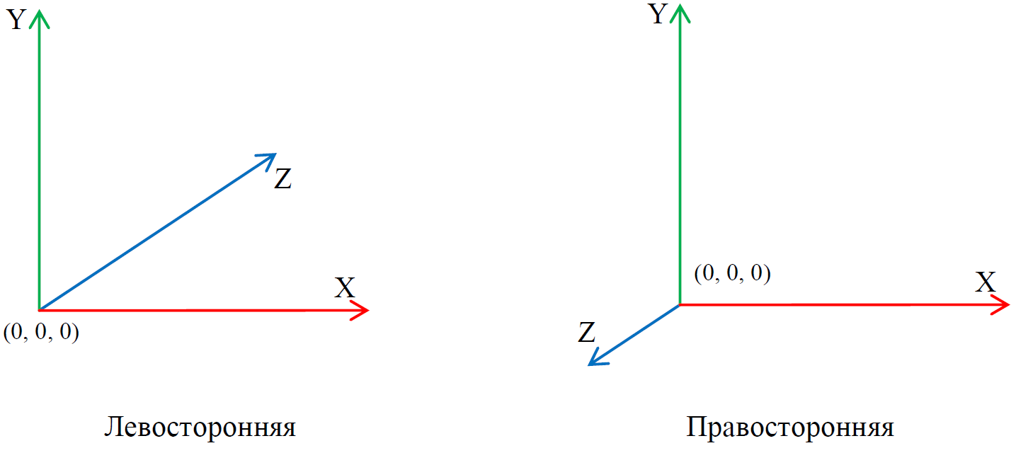
Fig. 2. Coordinate systems
As can be seen from fig. 2 coordinate systems differ only in the direction of the Z axis. OpenGL 1.0 actually uses the right-hand user coordinate system. But the CVV coordinate system and the user coordinate system are two completely different things. Moreover, since version 3.3, there is no longer such a thing as the standard OpenGL coordinate system. As mentioned earlier, the programmer himself implements the matrix operations module. The formation of rotation matrices, the formation of projection matrices, the search for the inverse matrix, the multiplication of matrices is the minimum set of operations included in the module of matrix operations. There are two logical questions. If the volume of visibility is a cube with an edge length equal to two, then why is a scene of several thousand conventional units visible on the screen? At what point is the translation of the user coordinate system into the CVV coordinate system. Projection matrices - this is the essence that deals with the solution of these issues.
The main idea of the foregoing is that the developer himself is free to choose the type of user coordinate system and must correctly describe the projection matrices. This completes the facts about OpenGL and it was time to bring it all together.
One of the most common and difficult to comprehend matrices is the perspective transformation matrix. So how is it related to CVV and user coordinate system? Why do objects become smaller with increasing distance to the observer? In order to understand why objects decrease with increasing distance, let's look at the matrix transformations of the three-dimensional model step by step. It is no secret that any three-dimensional model consists of a finite list of vertices that undergo matrix transformations completely independently of each other. In order to determine the coordinate of a three-dimensional vertex on a two-dimensional monitor screen it is necessary:
The translation of the Cartesian coordinates into a uniform coordinate was discussed earlier. The geometric meaning of the model matrix is to translate the model from the local coordinate system into the global coordinate system. Or, as they say, to bring the top of the model space in the world space. Let's just say, a three-dimensional object loaded from a file is in a model space, where the coordinates are counted relative to the object itself. Next, using the model matrix, the model is positioned, scaled, and rotated. As a result, all the vertices of the three-dimensional model receive the actual homogeneous coordinates in the three-dimensional scene. Model space relative to world space is local. From the model space, the coordinates are moved to world space (from local to global). For this, a model matrix is used.
Now go to step three. Here begins the species space. In this space, coordinates are counted relative to the position and orientation of the observer as if he were the center of the world. The species space is local relative to the world space, so the coordinates should be entered into it (and not carried out, as in the previous case). The direct matrix transformation takes the coordinates out of some space. To reverse them in it, it is necessary to invert the matrix transformation, therefore the species transformation is described by the inverse matrix. How to get this inverse matrix? First we get a direct matrix of the observer. What is characterized by an observer? The observer is described by the coordinate in which he is located, and the vectors of the direction of view. The observer is always looking in the direction of his local Z axis. The observer can move around the scene and make turns. In many ways, this is reminiscent of the meaning of the model matrix. By and large, the way it is. However, for an observer the scaling operation is meaningless, therefore, an equal sign cannot be put between the model matrix of the observer and the model matrix of a three-dimensional object. The model matrix of the observer is the desired direct matrix. Inverting this matrix, we get the view matrix. In practice, this means that all vertices in global homogeneous coordinates will receive new homogeneous coordinates relative to the observer. Accordingly, if the observer saw a certain vertex, then the value of the homogeneous z coordinate of the given vertex in the species space will be exactly a positive number. If the vertex was located behind the observer, then the value of its homogeneous coordinate z in the species space will be exactly a negative number.
Step four is the most interesting step. The previous steps were considered so deliberately in detail that the reader had a complete picture of all the operands of the fourth step. In the fourth step, homogeneous coordinates are removed from the species space into the CVV space. Once again, the fact is underlined that all potentially visible vertices will have a positive value of a uniform z coordinate.
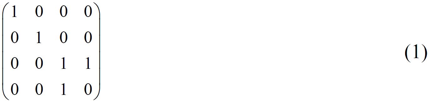
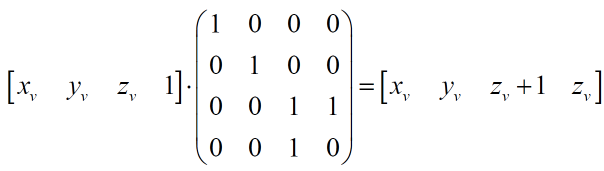
Consider a matrix of the form:
And a point in the homogeneous space of the observer:

We multiply the homogeneous coordinate by the matrix under consideration:
We translate the resulting homogeneous coordinates into Cartesian coordinates:
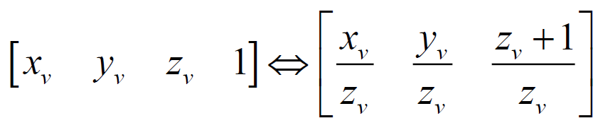
Suppose there are two points in the species space with the same x and y coordinates, but different z coordinates. In other words, one of the points is behind the other. Due to perspective distortion, the observer should see both points. Indeed, it is clear from the formula that, due to division by the z coordinate, compression occurs to the origin point. The greater the value of z (the farther the point is from the observer), the stronger the compression. Here is an explanation of the effect of perspective.
The OpenGL specification says that cutting and rasterization operations are performed in Cartesian coordinates, and the process of converting homogeneous coordinates to Cartesian coordinates is performed automatically.
The matrix (1) is the template for the matrix perspective of the projection. As mentioned earlier, the task of the projection matrix consists of two points: setting the user coordinate system (left or right), transferring the observer's visibility to the CVV. We derive the perspective matrix for the left-side user coordinate system.
The projection matrix can be described using four parameters (Fig. 3):
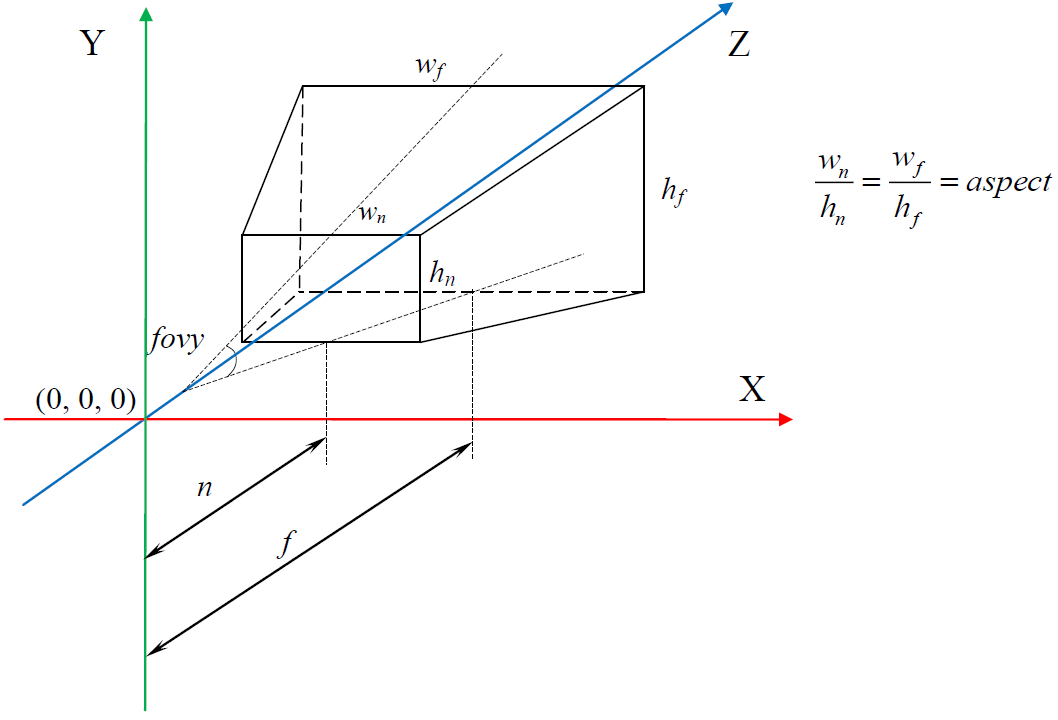
Fig. 3. Perspective visibility
Consider the projection of a point in the observer’s space onto the front cut-off face of the perspective visibility volume. For greater clarity in Fig. 4 shows a side view. It should also be noted that the user coordinate system coincides with the CVV coordinate system, that is, the left-side coordinate system is used everywhere.
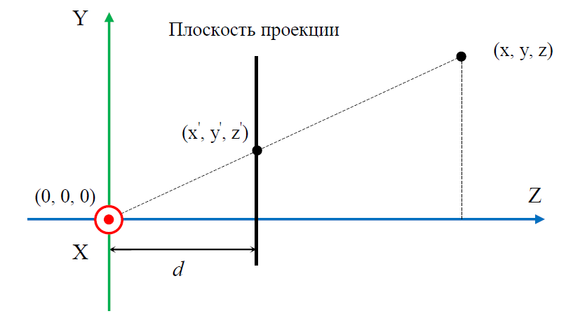
Fig. 4. Projecting an arbitrary point
Based on the properties of such triangles, the following equations are true:
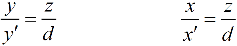
Express yꞌ and xꞌ:

In principle, expressions (2) are sufficient to obtain the coordinates of the points of the projection. However, for correct shielding of three-dimensional objects, it is necessary to know the depth of each fragment. In other words, it is necessary to store the value of the z component. This value is used in OpenGL depth tests. In fig. 3, it can be seen that the value of zꞌ is not suitable as a fragment depth, because all the projections of points can have the same value of zꞌ . The way out of this situation is the use of the so-called pseudo-depth.
Pseudo Depth Properties:
Let's derive the formula by which the pseudo depth will be calculated. As a basis, take the following expression:
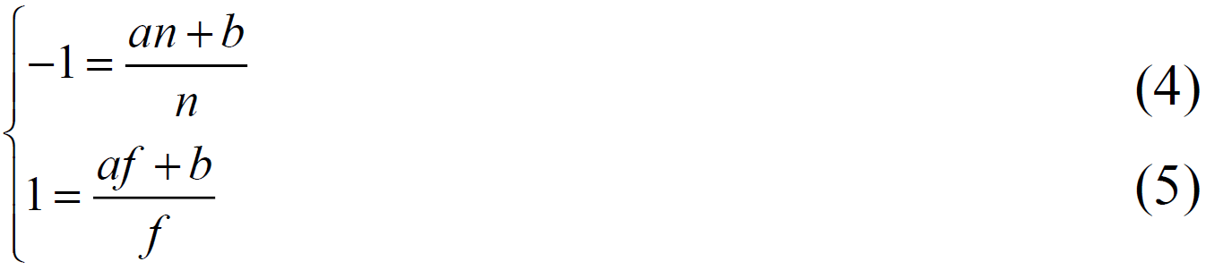
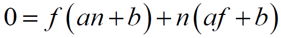
The coefficients a and b must be calculated. To do this, we use the properties of pseudo-depths 3 and 4. We obtain a system of two equations with two unknowns:
Make an addition of both parts of the system and multiply the result by the product fn , while f and n cannot equal zero. We get:
Open the brackets and rearrange the terms so that only the part with a remains on the left and only with b on the right:
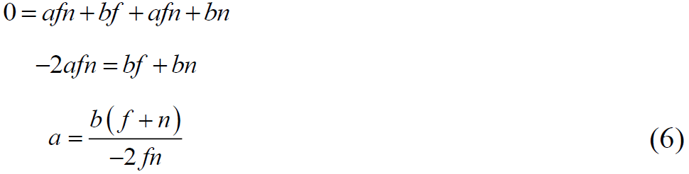
Substitute (6) into (5). We convert the expression to a simple fraction:
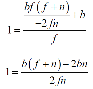
Multiply both sides by -2fn , while f and n cannot equal zero. We give similar, regroup the terms and express b :
Substitute (7) into (6) and express a :
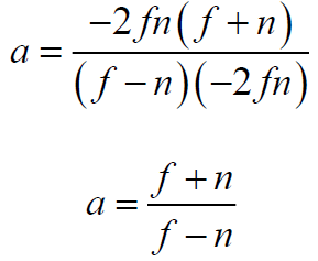
Accordingly, the components a and b are equal to:
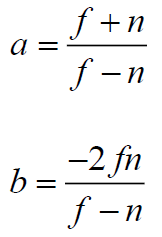
Now we substitute the obtained coefficients into the matrix blank (1) and see what happens with the z coordinate for an arbitrary point in a homogeneous observer space. The substitution is performed as follows:
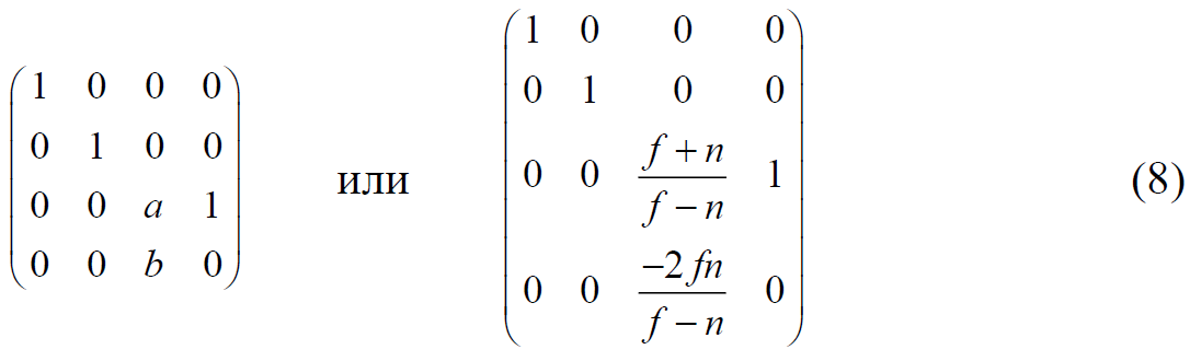
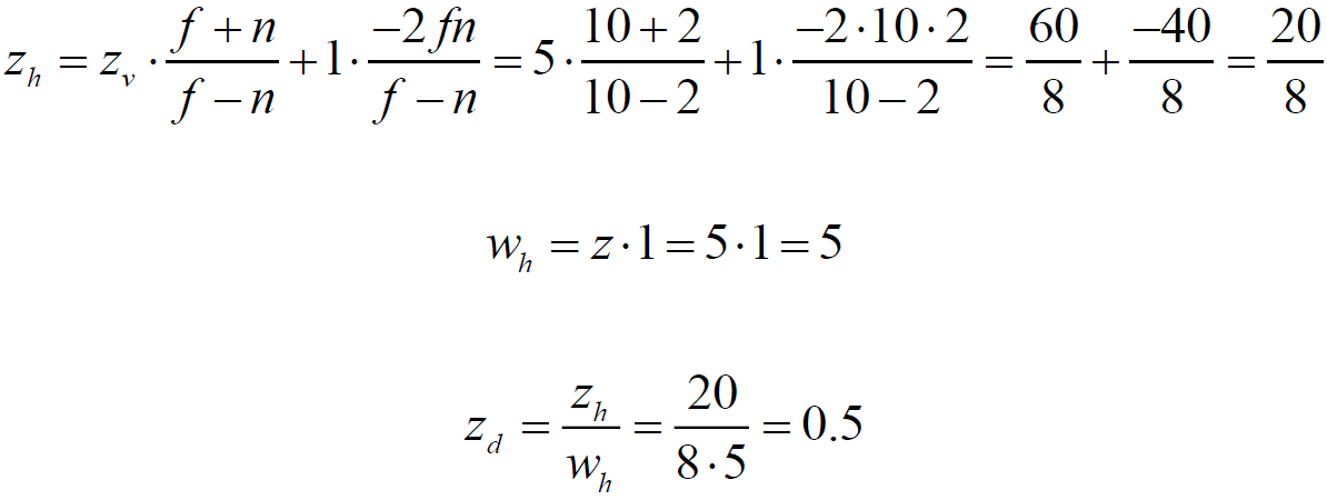
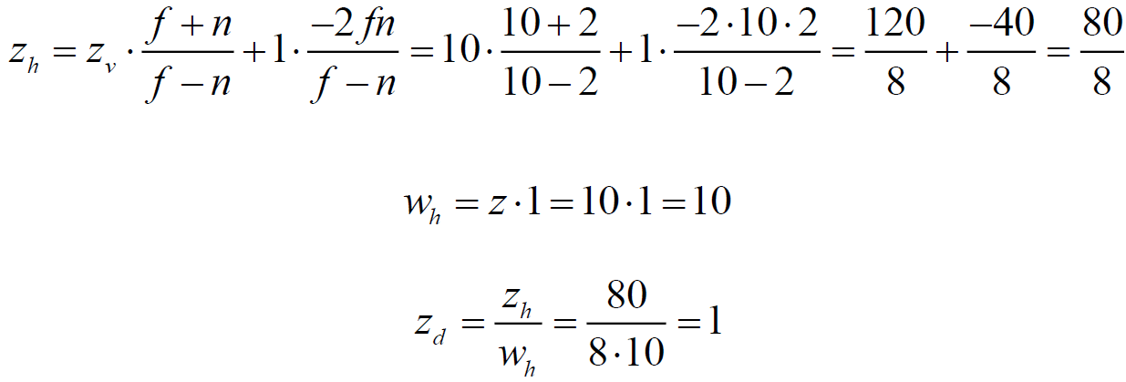
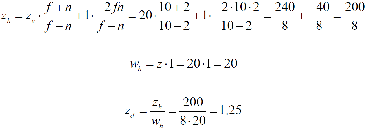
Let the distance to the front cut-off plane n be 2, and the distance to the far cut-off plane f be 10. Consider five points in the homogeneous observer space:
Multiply all points by the matrix (8), and then translate the resulting homogeneous coordinates into Cartesian coordinates . To do this, we need to calculate the values of the new homogeneous components.
  and
and  .
.
Point 1:
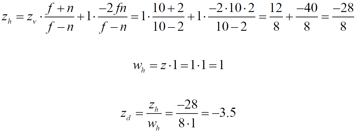
Point 2:
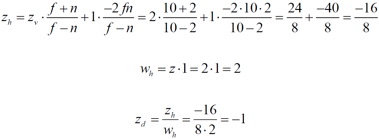
Point 3:
Point 4:
Point 5:
Note that the uniform coordinate absolutely true positioned in the CVV, and most importantly, that now the work of the OpenGL depth test is possible, because the pseudo depth fully satisfies the requirements of the tests.
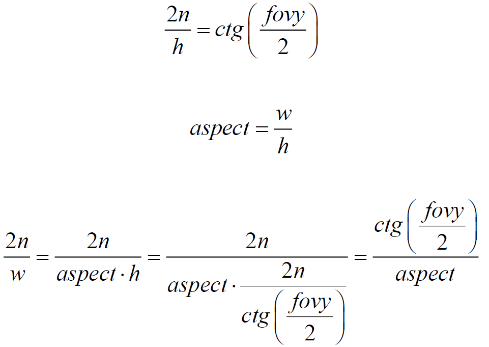
With the z coordinate figured out, move on to the coordinates x and y . As mentioned earlier, the entire prospective visibility volume should fit into the CVV. The CVV edge length is two. Accordingly, the height and width of the perspective visibility volume must be compressed to two conventional units.
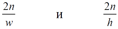
We have the fovy angle and the aspect value. Let's express the height and width using these values.
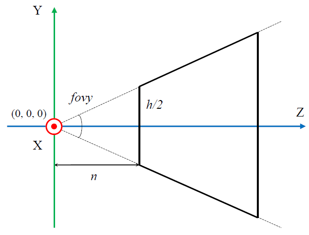
Fig. 5. Scope of visibility
From fig. 5 shows that:
Now you can get the final view of the perspective projection matrix for the user left-side coordinate system working with CVV OpenGL:

On this output matrix is complete.
A few words about DirectX - the main competitor of OpenGL. DirectX differs from OpenGL only in CVV dimensions and its positioning. In DirectX, CVV is a rectangular parallelepiped with lengths along the x and y axes equal to two, and along the z axis, the length is equal to one. The range of x and y is [-1 1], and the range of z is [0 1]. As for the CVV coordinate system, in DirectX, as in OpenGL, the left-sided coordinate system is used.
To display perspective matrices for a user-defined right-side coordinate system, it is necessary to redraw Fig. 2, Fig. 3 and Fig. 4, taking into account the new direction of the Z axis. Further, the calculations are completely analogous, up to a sign. For DirectX matrices, the pseudo-depth properties 3 and 4 are modified to the range [0 1].
On this topic of perspective matrices can be considered closed.
1. Graphics pipeline
2. Homogeneous coordinates
3. Lanterman A. Multicore and GPU programming for videogames
4. Lindeman RW CS 543 - Computer Graphics: Projection
5. Segal M., Akeley K. The OpenGL Graphics System: A Specification (Version 3.3 (Core Profile) - March 11, 2010)
6. Song HA OpenGL Projection Matrix
7. The OpenGL Shading Language Version 3.30
8. Tutorial 12 - Perspective Projection
9. Ignatenko A. Homogeneous coordinates
10. Perspective transformations
This is not a solution! Let's figure it out together!
Let's be realistic with a practical bias and take as an experimental OpenGL version 3.3. Starting with this version, each developer is obliged to independently implement the module of matrix operations. Great, this is what we need. Let's decompose ours with you a difficult task and highlight the main points. Some facts from the OpenGL specification:
- Matrices are stored in columns (column-major);
- Homogeneous coordinates;
- The canonical volume of clipping (CVV) in the left-side coordinate system.
There are two ways to store matrices: cool-major and row-major. In lectures on linear algebra, the row-major scheme is used. By and large, the representation of matrices in memory does not matter, because the matrix can always be translated into one type of representation into another by simple transposition. And if there is no difference, then for all subsequent calculations we will use the classic row-major matrices. When programming OpenGL, there is a small trick that allows you to abandon the transposition of matrices while maintaining the classic row-major calculations. In the shader program, the matrix needs to be transferred as it is, and in the shader it is necessary to multiply not the vector by the matrix, but the matrix by the vector.
')
Homogeneous coordinates is not a very tricky system with a number of simple rules for translating the usual Cartesian coordinates into homogeneous coordinates and back. The uniform coordinate is a [1x4] dimension row matrix. In order to translate the Cartesian coordinate into a homogeneous coordinate, x , y and z must be multiplied by any real number w (except 0). Next, you need to write the result in the first three components, and the last component will be equal to the factor w . In other words:
- Cartesian coordinatesw is a real number not equal to 0
- homogeneous coordinatesA little trick: If w is equal to one, then all that is needed for translation is to transfer the components x , y and z and assign the unit to the last component. That is, get the matrix row:
A few words about zero as w . From the point of view of homogeneous coordinates, this is quite permissible. Homogeneous coordinates allow you to distinguish points and vectors. In the Cartesian coordinate system, such a separation is impossible.
- point where ( x, y, z ) - Cartesian coordinates Is a vector, where ( x, y, z ) is a radius vectorThe reverse translation of a vertex from homogeneous coordinates to Cartesian coordinates is carried out as follows. All components of the matrix-row must be divided into the last component. In other words:
- homogeneous coordinates - Cartesian coordinatesThe main thing that you need to know is that all OpenGL algorithms for clipping and rasterization work in Cartesian coordinates, but before that, all the transformations are performed in homogeneous coordinates. The transition from homogeneous coordinates to Cartesian coordinates is carried out by hardware.
The canonical clipping volume or Canonic view volume (CVV) is one of the less documented parts of OpenGL. As can be seen from fig. 1 CVV is a cube aligned along the axes with the center at the origin and the edge length equal to two. Anything that enters the CVV area is subject to rasterization; anything outside the CVV is ignored. Anything that partially goes beyond CVV boundaries is subject to clipping algorithms. The most important thing to know is the CVV coordinate system is left-sided!
Fig. 1. OpenGL canonical clipping volume (CVV)
Left side coordinate system? How so, because in the OpenGL 1.0 specification it is clearly written that the coordinate system used is right-handed? Let's figure it out.
Fig. 2. Coordinate systems
As can be seen from fig. 2 coordinate systems differ only in the direction of the Z axis. OpenGL 1.0 actually uses the right-hand user coordinate system. But the CVV coordinate system and the user coordinate system are two completely different things. Moreover, since version 3.3, there is no longer such a thing as the standard OpenGL coordinate system. As mentioned earlier, the programmer himself implements the matrix operations module. The formation of rotation matrices, the formation of projection matrices, the search for the inverse matrix, the multiplication of matrices is the minimum set of operations included in the module of matrix operations. There are two logical questions. If the volume of visibility is a cube with an edge length equal to two, then why is a scene of several thousand conventional units visible on the screen? At what point is the translation of the user coordinate system into the CVV coordinate system. Projection matrices - this is the essence that deals with the solution of these issues.
The main idea of the foregoing is that the developer himself is free to choose the type of user coordinate system and must correctly describe the projection matrices. This completes the facts about OpenGL and it was time to bring it all together.
One of the most common and difficult to comprehend matrices is the perspective transformation matrix. So how is it related to CVV and user coordinate system? Why do objects become smaller with increasing distance to the observer? In order to understand why objects decrease with increasing distance, let's look at the matrix transformations of the three-dimensional model step by step. It is no secret that any three-dimensional model consists of a finite list of vertices that undergo matrix transformations completely independently of each other. In order to determine the coordinate of a three-dimensional vertex on a two-dimensional monitor screen it is necessary:
- Translate Cartesian coordinate to homogeneous coordinate;
- Multiply the uniform coordinate by the model matrix;
- The result is multiplied by the species matrix;
- The result is multiplied by the projection matrix;
- Result translate from homogeneous coordinates to Cartesian coordinates.
The translation of the Cartesian coordinates into a uniform coordinate was discussed earlier. The geometric meaning of the model matrix is to translate the model from the local coordinate system into the global coordinate system. Or, as they say, to bring the top of the model space in the world space. Let's just say, a three-dimensional object loaded from a file is in a model space, where the coordinates are counted relative to the object itself. Next, using the model matrix, the model is positioned, scaled, and rotated. As a result, all the vertices of the three-dimensional model receive the actual homogeneous coordinates in the three-dimensional scene. Model space relative to world space is local. From the model space, the coordinates are moved to world space (from local to global). For this, a model matrix is used.
Now go to step three. Here begins the species space. In this space, coordinates are counted relative to the position and orientation of the observer as if he were the center of the world. The species space is local relative to the world space, so the coordinates should be entered into it (and not carried out, as in the previous case). The direct matrix transformation takes the coordinates out of some space. To reverse them in it, it is necessary to invert the matrix transformation, therefore the species transformation is described by the inverse matrix. How to get this inverse matrix? First we get a direct matrix of the observer. What is characterized by an observer? The observer is described by the coordinate in which he is located, and the vectors of the direction of view. The observer is always looking in the direction of his local Z axis. The observer can move around the scene and make turns. In many ways, this is reminiscent of the meaning of the model matrix. By and large, the way it is. However, for an observer the scaling operation is meaningless, therefore, an equal sign cannot be put between the model matrix of the observer and the model matrix of a three-dimensional object. The model matrix of the observer is the desired direct matrix. Inverting this matrix, we get the view matrix. In practice, this means that all vertices in global homogeneous coordinates will receive new homogeneous coordinates relative to the observer. Accordingly, if the observer saw a certain vertex, then the value of the homogeneous z coordinate of the given vertex in the species space will be exactly a positive number. If the vertex was located behind the observer, then the value of its homogeneous coordinate z in the species space will be exactly a negative number.
Step four is the most interesting step. The previous steps were considered so deliberately in detail that the reader had a complete picture of all the operands of the fourth step. In the fourth step, homogeneous coordinates are removed from the species space into the CVV space. Once again, the fact is underlined that all potentially visible vertices will have a positive value of a uniform z coordinate.
Consider a matrix of the form:
And a point in the homogeneous space of the observer:
We multiply the homogeneous coordinate by the matrix under consideration:
We translate the resulting homogeneous coordinates into Cartesian coordinates:
Suppose there are two points in the species space with the same x and y coordinates, but different z coordinates. In other words, one of the points is behind the other. Due to perspective distortion, the observer should see both points. Indeed, it is clear from the formula that, due to division by the z coordinate, compression occurs to the origin point. The greater the value of z (the farther the point is from the observer), the stronger the compression. Here is an explanation of the effect of perspective.
The OpenGL specification says that cutting and rasterization operations are performed in Cartesian coordinates, and the process of converting homogeneous coordinates to Cartesian coordinates is performed automatically.
The matrix (1) is the template for the matrix perspective of the projection. As mentioned earlier, the task of the projection matrix consists of two points: setting the user coordinate system (left or right), transferring the observer's visibility to the CVV. We derive the perspective matrix for the left-side user coordinate system.
The projection matrix can be described using four parameters (Fig. 3):
- Viewing angle in radians ( fovy );
- Aspect ratio ( aspect );
- Distance to the near cut-off plane ( n );
- Distance to the far clipping plane ( f ).
Fig. 3. Perspective visibility
Consider the projection of a point in the observer’s space onto the front cut-off face of the perspective visibility volume. For greater clarity in Fig. 4 shows a side view. It should also be noted that the user coordinate system coincides with the CVV coordinate system, that is, the left-side coordinate system is used everywhere.
Fig. 4. Projecting an arbitrary point
Based on the properties of such triangles, the following equations are true:
Express yꞌ and xꞌ:
In principle, expressions (2) are sufficient to obtain the coordinates of the points of the projection. However, for correct shielding of three-dimensional objects, it is necessary to know the depth of each fragment. In other words, it is necessary to store the value of the z component. This value is used in OpenGL depth tests. In fig. 3, it can be seen that the value of zꞌ is not suitable as a fragment depth, because all the projections of points can have the same value of zꞌ . The way out of this situation is the use of the so-called pseudo-depth.
Pseudo Depth Properties:
- The pseudo depth is calculated based on the value of z ;
- The closer the point is to the observer, the smaller the pseudo depth is;
- For all points lying on the front plane of the scope, the pseudo depth is -1;
- For all points lying in the far plane of the cut-off of the scope of visibility, the pseudo depth value is 1;
- All fragments that lie within the scope of visibility have a pseudo-depth value in the range [-1 1].
Let's derive the formula by which the pseudo depth will be calculated. As a basis, take the following expression:
The coefficients a and b must be calculated. To do this, we use the properties of pseudo-depths 3 and 4. We obtain a system of two equations with two unknowns:
Make an addition of both parts of the system and multiply the result by the product fn , while f and n cannot equal zero. We get:
Open the brackets and rearrange the terms so that only the part with a remains on the left and only with b on the right:
Substitute (6) into (5). We convert the expression to a simple fraction:
Multiply both sides by -2fn , while f and n cannot equal zero. We give similar, regroup the terms and express b :
Substitute (7) into (6) and express a :
Accordingly, the components a and b are equal to:
Now we substitute the obtained coefficients into the matrix blank (1) and see what happens with the z coordinate for an arbitrary point in a homogeneous observer space. The substitution is performed as follows:
Let the distance to the front cut-off plane n be 2, and the distance to the far cut-off plane f be 10. Consider five points in the homogeneous observer space:
| Point | Value | Description |
|---|---|---|
| one | one | The point is in front of the front cut-off visibility plane. Does not pass rasterization. |
| 2 | 2 | The point is located on the front edge of the cut-off volume of visibility. Pass rasterization. |
| 3 | five | The point is located between the front edge of the cut-off and the far edge of the cut-off volume of visibility. Pass rasterization. |
| four | ten | The point is on the far edge of the cut-off volume of visibility. Pass rasterization. |
| five | 20 | The point is beyond the far edge of the cut-off visibility. Does not pass rasterization. |
Multiply all points by the matrix (8), and then translate the resulting homogeneous coordinates into Cartesian coordinates
Point 1:
Point 2:
Point 3:
Point 4:
Point 5:
Note that the uniform coordinate
With the z coordinate figured out, move on to the coordinates x and y . As mentioned earlier, the entire prospective visibility volume should fit into the CVV. The CVV edge length is two. Accordingly, the height and width of the perspective visibility volume must be compressed to two conventional units.
We have the fovy angle and the aspect value. Let's express the height and width using these values.
Fig. 5. Scope of visibility
From fig. 5 shows that:
Now you can get the final view of the perspective projection matrix for the user left-side coordinate system working with CVV OpenGL:
On this output matrix is complete.
A few words about DirectX - the main competitor of OpenGL. DirectX differs from OpenGL only in CVV dimensions and its positioning. In DirectX, CVV is a rectangular parallelepiped with lengths along the x and y axes equal to two, and along the z axis, the length is equal to one. The range of x and y is [-1 1], and the range of z is [0 1]. As for the CVV coordinate system, in DirectX, as in OpenGL, the left-sided coordinate system is used.
To display perspective matrices for a user-defined right-side coordinate system, it is necessary to redraw Fig. 2, Fig. 3 and Fig. 4, taking into account the new direction of the Z axis. Further, the calculations are completely analogous, up to a sign. For DirectX matrices, the pseudo-depth properties 3 and 4 are modified to the range [0 1].
On this topic of perspective matrices can be considered closed.
Useful literature
1. Graphics pipeline
2. Homogeneous coordinates
3. Lanterman A. Multicore and GPU programming for videogames
4. Lindeman RW CS 543 - Computer Graphics: Projection
5. Segal M., Akeley K. The OpenGL Graphics System: A Specification (Version 3.3 (Core Profile) - March 11, 2010)
6. Song HA OpenGL Projection Matrix
7. The OpenGL Shading Language Version 3.30
8. Tutorial 12 - Perspective Projection
9. Ignatenko A. Homogeneous coordinates
10. Perspective transformations
Source: https://habr.com/ru/post/252771/
All Articles