Entertaining math in Hearthstone
I am a fan of the popular computer card game Hearthstone, developed by Blizzard Entertainment. Once I asked myself a question: “Is it possible, based only on the rules describing the dynamics of a player’s transition between levels when a player loses / wins, to get statistics on the distribution of players by the level they reached?”
Despite the fact that the network has a huge number of sites and wiki dedicated to Hearthstone, superficial search did not give any results. It was a pity for the deep search, so I solved the problem “on the knee”. I suppose this decision can be a topic for classes in a school math circle.
In the Hearthstone ranking tournament there are 25 levels and a special Legend level. Levels consist of sublevels - the so-called. "Stars", and at different levels the number of sublevels is different:
Thus, the level ruler in the rating (hereinafter referred to as the ruler) consists of 96 sublevels (including the “Legend”):
')

Picture 1
The new player starts in the ranking from the 25th level. For winning a game, a player gets a “star” (sometimes two), i.e. Increases its sublevel by 1 (or 2, respectively).
There are 4 ranges on the ruler, in which the rules for changing the player’s level when winning / losing a game are different:
Table 1
Obviously, “Springboard” serves to involve new players, since there is only a reward on the “springboard”, but there is no punishment for defeat. In addition, it is clear that the population of the "springboard" exponentially quickly "dies out", since the rules inevitably push the player from the "springboard" into the range of "Race with acceleration". The probability of remaining on the “springboard” after 18 games is ~ 29%, and after 27 games - less than 1.5%.
"Race with acceleration" helps players with high skill and good decks to quickly get to the "Normal Race", where the real "ruble" begins. And finally, the Legend is a pin for top players.
I wanted to find 2 dependencies:
The first thought was to write a JS program that simulates a multitude of players whose levels change as a result of the interaction according to the above rules. After a brief reflection on the size of the required JS code, I decided that spreadsheets are excellent for this task.
The solution is as follows:
Let some rectangular range with the size of 96 * 1 (for example, the Source! $ C $ 3: $ C $ 98 range in the attached files) represent the distribution of the number of players in the line. Then, using the rules from table 1, it is easy to obtain a distribution describing the state after each player has played one game. The rules in Table 1 are located in the Source! $ D3: $ D $ 98 range. If you “push” these rules to the required number of columns, the resulting table will represent the change in the distribution of players in levels with “time”. Time in this case is in quotes because here it is measured in “games played”.
I started with Open Office Calc, which is good for everyone, but the 3-D graphics out of the box look poor in it (maybe I just don’t know how to prepare them). As a result, the solution is implemented in MS Excel and lies here . The option for Open Office Calc in the same place is quite functional, except for the absence of 3-D graphs and the lack of interactivity in 2-D graphs.
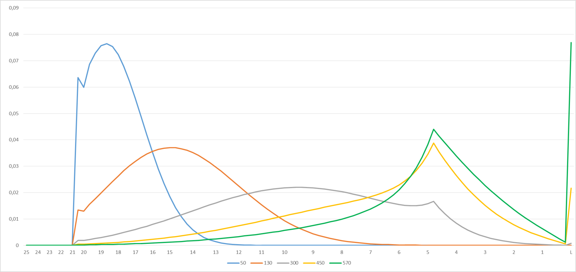
Figure 2
The given charts describe the probability of getting this or that level for a player who started from level 25 and played 50, 130, 300, 450 or 570 games respectively. In Excel, the graph is interactive - you can play around with the numbers to the left of the diagram on the Interface tab, and the graphs (Figure 2) will change.
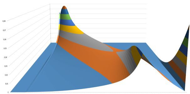
In the 3-D evolution of the probability of obtaining a certain level looks very nice:
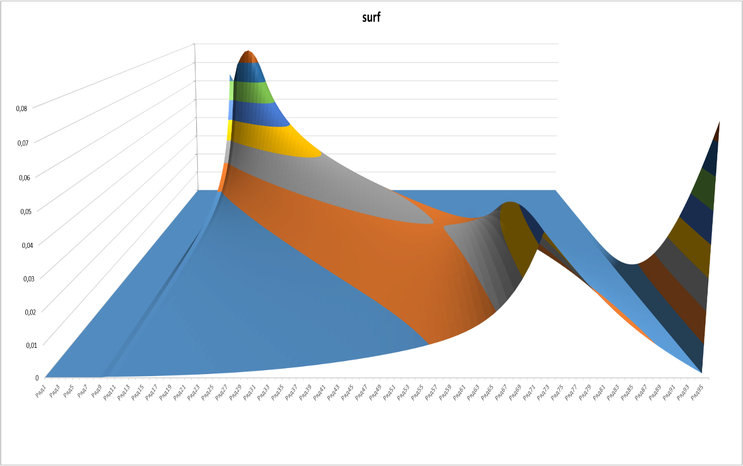
Figure 3
Here is a slice with the same minimum and maximum "temporary" boundaries (50 and 570 games), as in Figure 2.
The same graph from another angle:
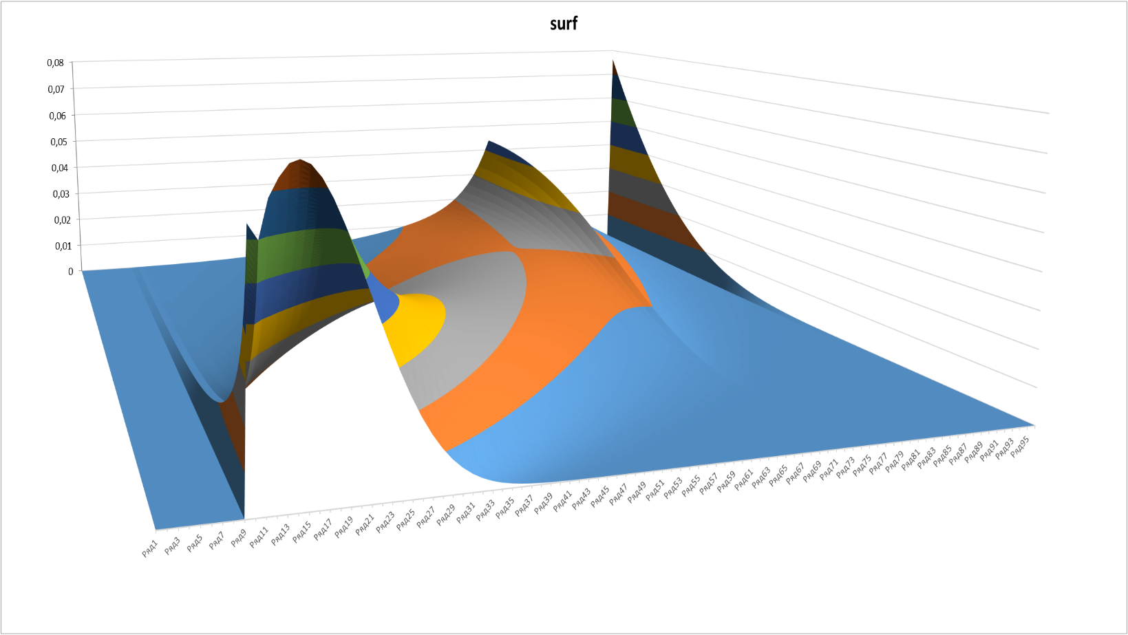
Figure 4
The appearance of the “edge” on the graphs at the point corresponding to the level 5 and 2 of the “star” looks somewhat unexpected (72nd sublevel in order). This point is the last, which is affected by the possibility of “accelerating” after 3+ victories in a row.
If you look at the rules for 71 - 72 sublevels, then they look like this:
71 = 1/8 * C69 + C70 * 3/8 + 0.5 * C72
72 = 1/8 * C70 + C71 * 1/2 + 0.5 * C73
Here CNN is the number of players at the NN sublevel in the previous step:
- the first member provides “accelerated transfer” from the “current -2” level;
- the second member provides the usual transition when winning at the “current -1” level;
- the third member provides a transition from the upper level with the defeat.
The difference in 1/8 in the coefficient for the second term is due to the fact that, starting from the 5th level (it is the 71st ordinal sublevel), regardless of the number of victories in a row, the sublevel increases only by 1, i.e. even if the victory on the 71st sublevel was for the 3rd player, he will go only to the 72nd sublevel.
This small, at first glance, additive leads to the fact that the “flow of players” to the 72nd sublevel is slightly above average, respectively, the flow of players from the 72nd sublevel to its neighborhood, i.e. the effect of increasing the flow of players to the 72nd sublevel is self-reinforcing, which leads to the appearance of this remarkable edge.
Obviously, players differ in the number of games they play in the same time. More enthusiastic players play more, casual less.
To calculate the model distribution of players by levels, it is necessary to know the distribution function of players by the number of games played by them.
We introduce the notation:
Then
At once I will say that I have no data on the function Z (i, N). But you can speculate on this topic.
The only thing that occurred to me was: “20% of people drink 80% of beer”. Perhaps "20% of Hearthstone players play 80% of the games"? That is, the hypothesis is that the distribution of players by the number of games played is a discrete Pareto distribution, or, more precisely, a Zipf distribution (see en.wikipedia.org/wiki/Zipf%27s_law ).
We introduce the notation:
Then the Zipf distribution with power exponent s:

Let's look at the graphs of the desired function D (L, N) under the assumption that the distribution of players by the number of games played is a Zipf distribution with exponent 1.
Here and in the following graph, D (L, N) is displayed at times of “time” N from 50 to 700.
Figure 5
Figure 6
It looks rather ugly, although it is understandable why - a significant part of the players, in accordance with the Zipf distribution, remained on the “springboard”. Well, to speculate - so in full. We construct a modified Zipf-Mandelbrot distribution (see en.wikipedia.org/wiki/Zipf%E2%80%93Mandelbrot_law ).
1. Replace the auxiliary function
The idea of introducing the Startshift integer parameter is as follows: the beginning of the “action” of the standard behavior of the Zipf distribution is shifted by the Startshift steps.
Indeed, it seems implausible that a player who has undergone all the difficulties of learning and who has just entered the rating games, is more likely to stop playing after one or two rating games. It can be assumed that the beginning of the “action” of the Zipf distribution roughly coincides with the onset of difficulties in advancing in the rating, i.e. with the moment when the probability of leaving the "springboard" exceeds ½ (this means that startshift = 18). In addition, the definition of the auxiliary function implies that the total number of players who “accidentally entered Hearthstone” (i.e. played ≤ Startshift games) coincides with the number of players at the maximum distribution. All this, of course, pure speculation, but why not see what happens?
The Mandelbrot parameter q is entered without any justification, just in case.
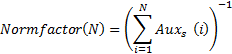
2. The normalization factor (for the moment of "time" N)
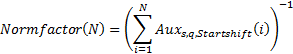
Then a modified distribution with a power exponent s, the Mandelbrot parameter q and the Startshift "start shift" parameter:

Let's see what happens with the parameters shown at the bottom of the chart:
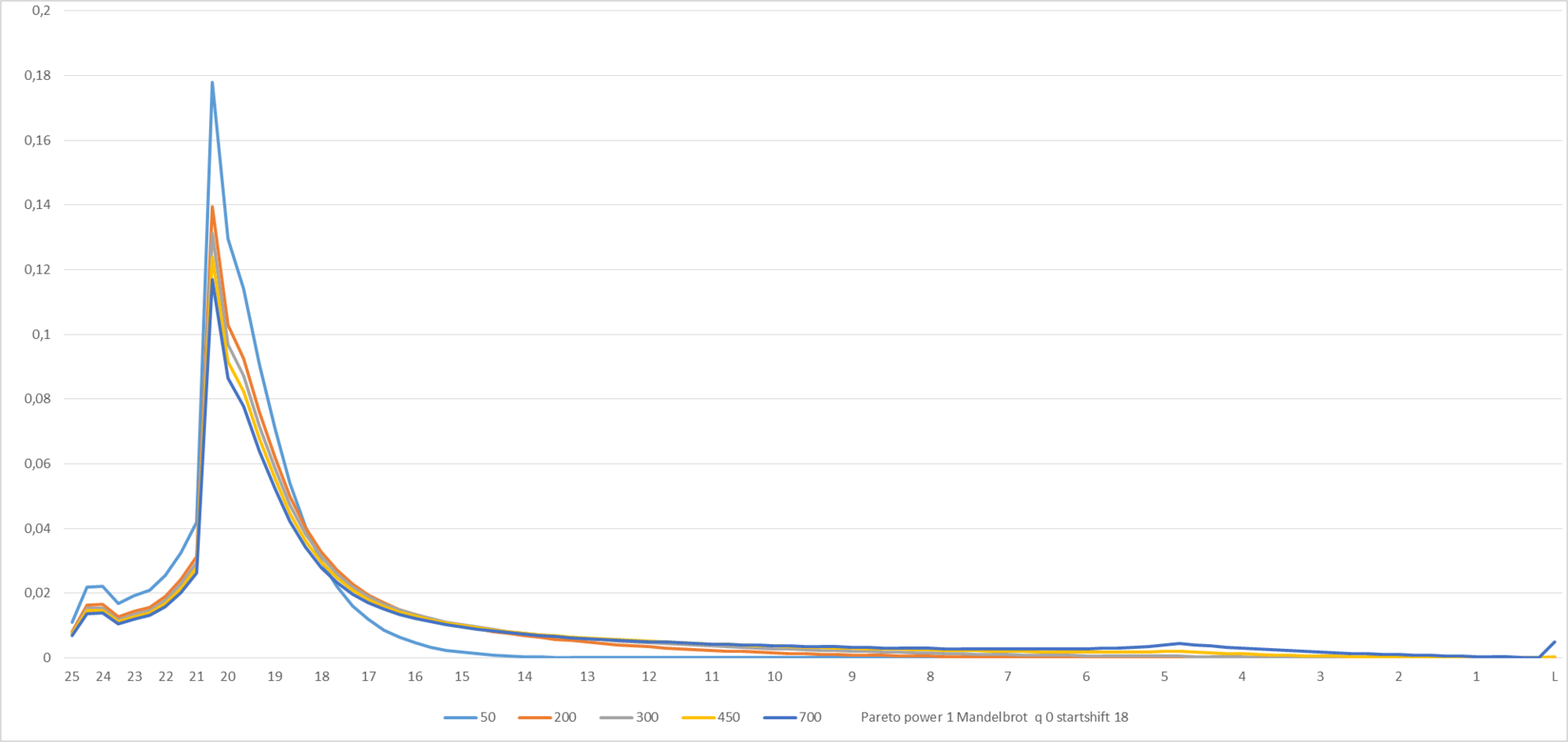
Figure 7
For manual experiments, the graph in Excel is made interactive - you can play around with the distribution parameters and the displayed “times” to the left of the diagram on the Interface tab, and the graphs (Figure 7 and Figure 8) will change.
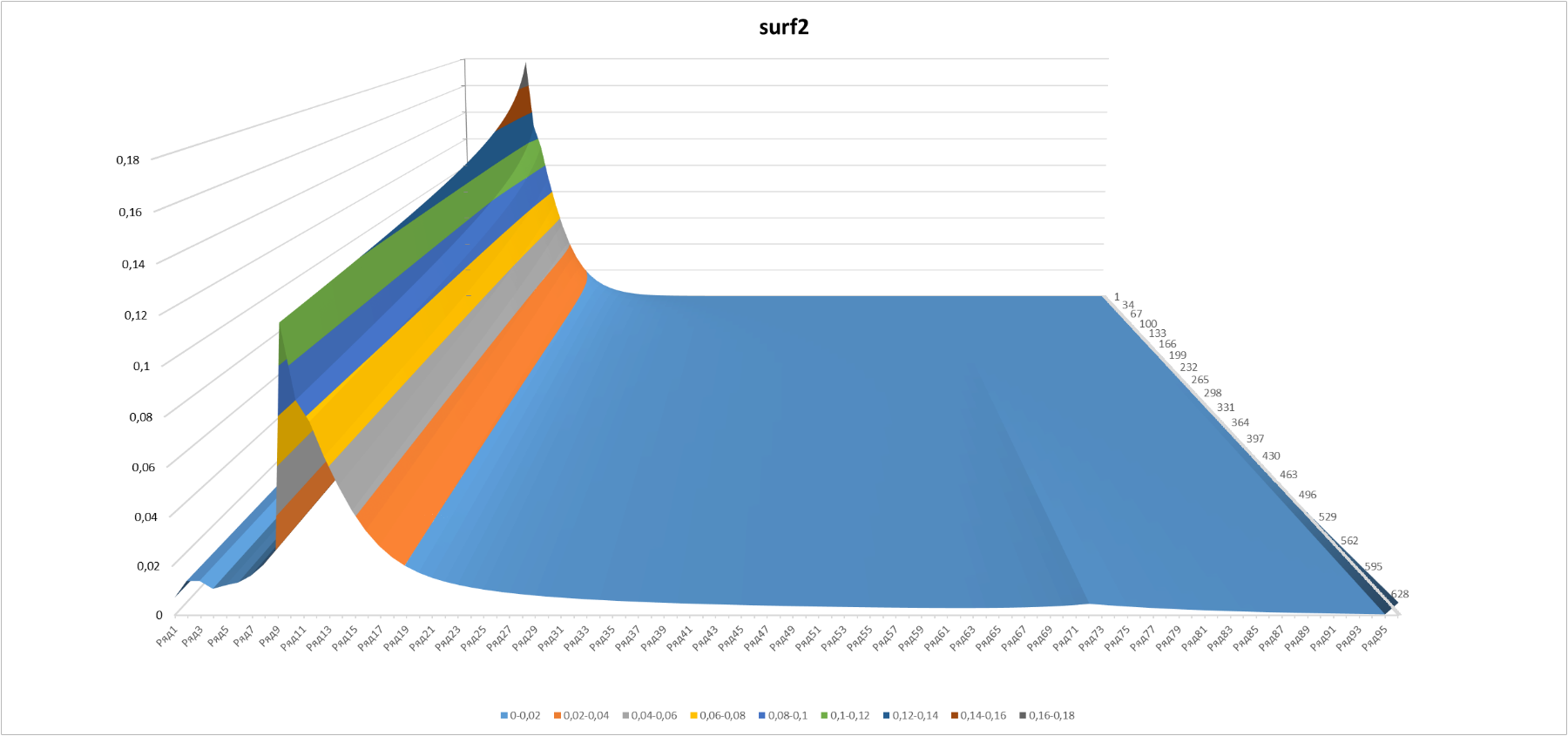
Figure 8
And finally, the last spurt for today. Let's try to choose distribution parameters using “real” data (http://www.reddit.com/r/hearthstone/comments/23ed7l/how_good_are_you_at_constructed_ladder/). These are the results of some kind of simulation, the details of which are unknown to me, it is unclear, in particular, at what point in the “time” N the measurement was taken, etc. This is the only thing I found. But I did not really try to look. Hopefully, readers of the article will prompt a source of more relevant data.
Iterative processing of data by the solver add-in and manual adjustment gave the following values of the distribution parameters: s = 1.19; q = 0,287; Startshift = 110. Startshift is expectedly large, since there is no information about population levels 25-21 in the initial simulation data, i.e. "Springboard", obviously, was not simulated.
Final pictures:
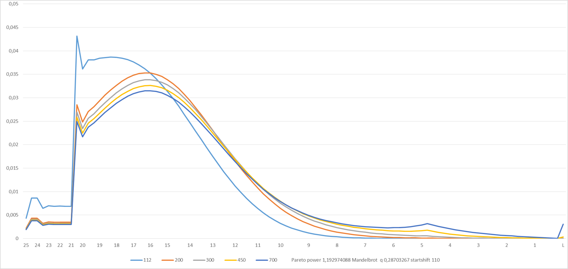
Figure 9
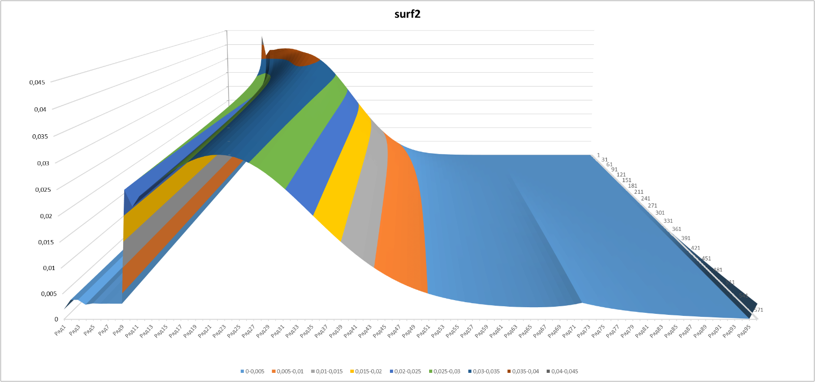
Figure 10
In conclusion, I repeat that the task that I began to solve out of pure curiosity seemed to me a good topic for studying in a school math group. I consider it important for future engineers and scientists to be able to use all available tools at hand for solving sudden problems, such as paper and pencil, spreadsheets, and the WOLFRAM MATHEMATICA package. I hope this example of applying a spreadsheet will be useful to someone.
If desired, the teacher can build bridges from this task to a variety of topics.
Offhand:
You can also come up with some extensions to this task. For example, such:
1) When the season ends, players who have reached certain levels in the last season get some odds. For example, at the end of a season at level 4, a player gets 21 "stars", i.e. starts in the new season not from level 25, but from level 17. ** - it’s the 21st ordinal level (see Figure 1). I am sure that the corresponding figures describing the dependence of the size of the odds on the achieved level can be easily found on the network.
Questions:
2) Come up with some clear theory to calculate the function Z (i, N).
Despite the fact that the network has a huge number of sites and wiki dedicated to Hearthstone, superficial search did not give any results. It was a pity for the deep search, so I solved the problem “on the knee”. I suppose this decision can be a topic for classes in a school math circle.
Task Description
In the Hearthstone ranking tournament there are 25 levels and a special Legend level. Levels consist of sublevels - the so-called. "Stars", and at different levels the number of sublevels is different:
- Levels 25 through 21 consist of 2 sublevels;
- Levels 20 through 16 consist of 3 sublevels;
- Levels 15 through 11 consist of 4 sublevels;
- Levels 10 through 1 consist of 5 sublevels;
- There are no sublevels on Legend.
Thus, the level ruler in the rating (hereinafter referred to as the ruler) consists of 96 sublevels (including the “Legend”):
')
Picture 1
The new player starts in the ranking from the 25th level. For winning a game, a player gets a “star” (sometimes two), i.e. Increases its sublevel by 1 (or 2, respectively).
There are 4 ranges on the ruler, in which the rules for changing the player’s level when winning / losing a game are different:
Table 1
| Code name | Level range | Rules for changing the sublevel when winning / losing |
|---|---|---|
| "Springboard" | 25-21 | Defeat: sublevel does not change Victory: +1 3 (and more) victories in a row: +2 |
| "Race with acceleration" | 20-6 | Damage: -1 Victory: +1 3 (and more) victories in a row: +2 |
| "Normal race" | 5-1 | Damage: -1 Victory: +1 |
| "Legend" | Legend | Defeat: sublevel does not change Victory: the sublayer does not change |
Obviously, “Springboard” serves to involve new players, since there is only a reward on the “springboard”, but there is no punishment for defeat. In addition, it is clear that the population of the "springboard" exponentially quickly "dies out", since the rules inevitably push the player from the "springboard" into the range of "Race with acceleration". The probability of remaining on the “springboard” after 18 games is ~ 29%, and after 27 games - less than 1.5%.
"Race with acceleration" helps players with high skill and good decks to quickly get to the "Normal Race", where the real "ruble" begins. And finally, the Legend is a pin for top players.
I wanted to find 2 dependencies:
- Calculate the probability of a player getting a certain level after a certain number of games played;
- Calculate the distribution of all players by level depending on time.
Choosing a solution method and tool
The first thought was to write a JS program that simulates a multitude of players whose levels change as a result of the interaction according to the above rules. After a brief reflection on the size of the required JS code, I decided that spreadsheets are excellent for this task.
The solution is as follows:
Let some rectangular range with the size of 96 * 1 (for example, the Source! $ C $ 3: $ C $ 98 range in the attached files) represent the distribution of the number of players in the line. Then, using the rules from table 1, it is easy to obtain a distribution describing the state after each player has played one game. The rules in Table 1 are located in the Source! $ D3: $ D $ 98 range. If you “push” these rules to the required number of columns, the resulting table will represent the change in the distribution of players in levels with “time”. Time in this case is in quotes because here it is measured in “games played”.
I started with Open Office Calc, which is good for everyone, but the 3-D graphics out of the box look poor in it (maybe I just don’t know how to prepare them). As a result, the solution is implemented in MS Excel and lies here . The option for Open Office Calc in the same place is quite functional, except for the absence of 3-D graphs and the lack of interactivity in 2-D graphs.
The probability of a player getting a certain level
Figure 2
The given charts describe the probability of getting this or that level for a player who started from level 25 and played 50, 130, 300, 450 or 570 games respectively. In Excel, the graph is interactive - you can play around with the numbers to the left of the diagram on the Interface tab, and the graphs (Figure 2) will change.
In the 3-D evolution of the probability of obtaining a certain level looks very nice:
Figure 3
Here is a slice with the same minimum and maximum "temporary" boundaries (50 and 570 games), as in Figure 2.
The same graph from another angle:
Figure 4
The appearance of the “edge” on the graphs at the point corresponding to the level 5 and 2 of the “star” looks somewhat unexpected (72nd sublevel in order). This point is the last, which is affected by the possibility of “accelerating” after 3+ victories in a row.
If you look at the rules for 71 - 72 sublevels, then they look like this:
71 = 1/8 * C69 + C70 * 3/8 + 0.5 * C72
72 = 1/8 * C70 + C71 * 1/2 + 0.5 * C73
Here CNN is the number of players at the NN sublevel in the previous step:
- the first member provides “accelerated transfer” from the “current -2” level;
- the second member provides the usual transition when winning at the “current -1” level;
- the third member provides a transition from the upper level with the defeat.
The difference in 1/8 in the coefficient for the second term is due to the fact that, starting from the 5th level (it is the 71st ordinal sublevel), regardless of the number of victories in a row, the sublevel increases only by 1, i.e. even if the victory on the 71st sublevel was for the 3rd player, he will go only to the 72nd sublevel.
This small, at first glance, additive leads to the fact that the “flow of players” to the 72nd sublevel is slightly above average, respectively, the flow of players from the 72nd sublevel to its neighborhood, i.e. the effect of increasing the flow of players to the 72nd sublevel is self-reinforcing, which leads to the appearance of this remarkable edge.
Calculate the distribution of all players by level
Obviously, players differ in the number of games they play in the same time. More enthusiastic players play more, casual less.
To calculate the model distribution of players by levels, it is necessary to know the distribution function of players by the number of games played by them.
We introduce the notation:
- P (L, i)) - the probability of a player getting a certain level (L) after a specified number of games (i) (graphs are shown in Figures 2-4)
- N - the maximum number of games played by the most enthusiastic player. Note that N plays the role of time here. Of course, this is not the usual time. However, between the usual time t and N there is the following relationship:
 therefore, N as a “time” is quite suitable.
 - Z (i, N) is the probability that a player has played i games by the time “time” N or the distribution of players by the number of games played in “time” N.
- D (L, N) - the desired probability of finding a player at level L, at the time of "time" N or the distribution of players in levels at the time of "time" N.
Then
At once I will say that I have no data on the function Z (i, N). But you can speculate on this topic.
The only thing that occurred to me was: “20% of people drink 80% of beer”. Perhaps "20% of Hearthstone players play 80% of the games"? That is, the hypothesis is that the distribution of players by the number of games played is a discrete Pareto distribution, or, more precisely, a Zipf distribution (see en.wikipedia.org/wiki/Zipf%27s_law ).
We introduce the notation:
- Auxiliary function

- Normalization factor (for the moment of "time" N)
Then the Zipf distribution with power exponent s:
Let's look at the graphs of the desired function D (L, N) under the assumption that the distribution of players by the number of games played is a Zipf distribution with exponent 1.
Here and in the following graph, D (L, N) is displayed at times of “time” N from 50 to 700.
Figure 5
Figure 6
It looks rather ugly, although it is understandable why - a significant part of the players, in accordance with the Zipf distribution, remained on the “springboard”. Well, to speculate - so in full. We construct a modified Zipf-Mandelbrot distribution (see en.wikipedia.org/wiki/Zipf%E2%80%93Mandelbrot_law ).
1. Replace the auxiliary function
The idea of introducing the Startshift integer parameter is as follows: the beginning of the “action” of the standard behavior of the Zipf distribution is shifted by the Startshift steps.
Indeed, it seems implausible that a player who has undergone all the difficulties of learning and who has just entered the rating games, is more likely to stop playing after one or two rating games. It can be assumed that the beginning of the “action” of the Zipf distribution roughly coincides with the onset of difficulties in advancing in the rating, i.e. with the moment when the probability of leaving the "springboard" exceeds ½ (this means that startshift = 18). In addition, the definition of the auxiliary function implies that the total number of players who “accidentally entered Hearthstone” (i.e. played ≤ Startshift games) coincides with the number of players at the maximum distribution. All this, of course, pure speculation, but why not see what happens?
The Mandelbrot parameter q is entered without any justification, just in case.
2. The normalization factor (for the moment of "time" N)
Then a modified distribution with a power exponent s, the Mandelbrot parameter q and the Startshift "start shift" parameter:
Let's see what happens with the parameters shown at the bottom of the chart:
Figure 7
For manual experiments, the graph in Excel is made interactive - you can play around with the distribution parameters and the displayed “times” to the left of the diagram on the Interface tab, and the graphs (Figure 7 and Figure 8) will change.
Figure 8
And finally, the last spurt for today. Let's try to choose distribution parameters using “real” data (http://www.reddit.com/r/hearthstone/comments/23ed7l/how_good_are_you_at_constructed_ladder/). These are the results of some kind of simulation, the details of which are unknown to me, it is unclear, in particular, at what point in the “time” N the measurement was taken, etc. This is the only thing I found. But I did not really try to look. Hopefully, readers of the article will prompt a source of more relevant data.
Iterative processing of data by the solver add-in and manual adjustment gave the following values of the distribution parameters: s = 1.19; q = 0,287; Startshift = 110. Startshift is expectedly large, since there is no information about population levels 25-21 in the initial simulation data, i.e. "Springboard", obviously, was not simulated.
Final pictures:
Figure 9
Figure 10
Conclusion
In conclusion, I repeat that the task that I began to solve out of pure curiosity seemed to me a good topic for studying in a school math group. I consider it important for future engineers and scientists to be able to use all available tools at hand for solving sudden problems, such as paper and pencil, spreadsheets, and the WOLFRAM MATHEMATICA package. I hope this example of applying a spreadsheet will be useful to someone.
If desired, the teacher can build bridges from this task to a variety of topics.
Offhand:
- Theorver - Pareto distribution - Zeta function - John Derbyshire. Prime Obsession: Bernhard Riemann and the Greatest Unsolved Problem in Mathematics
- Numerical methods for solving partial differential derivatives. (by the way - a task for advanced students: show that P (L, i) in the “Normal Race” range approximates some particular solution of the equation
 in the appropriate scale, and in the “Race with Acceleration” range - the equations
- Selection of the type of residual function optimal for the problem.
You can also come up with some extensions to this task. For example, such:
1) When the season ends, players who have reached certain levels in the last season get some odds. For example, at the end of a season at level 4, a player gets 21 "stars", i.e. starts in the new season not from level 25, but from level 17. ** - it’s the 21st ordinal level (see Figure 1). I am sure that the corresponding figures describing the dependence of the size of the odds on the achieved level can be easily found on the network.
Questions:
- How will P (L, i) and D (L, N) change when taking into account the odds at the start of the season?
- Does a series of functions D (L, N, season number) match anything with a season number tending to ∞? If so, what restrictions does this impose on Z (i, N)?
- Is Z (i, N) enough for a correct answer to the 2nd question?
2) Come up with some clear theory to calculate the function Z (i, N).
Source: https://habr.com/ru/post/252713/
All Articles