Machine learning - 2. Nonlinear regression and numerical optimization
A month has passed since the appearance of my first article on Habré and 20 days since the appearance of the second article about linear regression . Statistics on views and target actions of the audience is accumulated, and it was this that served as the starting point for this article. In it, we will briefly review an example of nonlinear regression (namely, exponential) and use it to build a conversion model, highlighting two groups among users.
When it is known that the random variable y depends on something (for example, on time or on another random variable x) linearly, i.e. According to the law y (x) = Ax + b, linear regression is applied (as in the previous article, we built the dependence of the number of registrations on the number of views). For linear regression, the coefficients A and b are calculated using the known formulas. In the case of another type of regression, for example, exponential, in order to determine the unknown parameters, it is necessary to solve the corresponding optimization problem: namely, in the framework of the least squares method (OLS), the problem of finding the minimum of the sum of squares (y (x i ) - y i ) 2 .
So, here are the data that we will use as an example. Attendance peaks (Views row, red dotted line) are at the time of publication of articles. The second data series (Regs, with a multiplier of 100) shows the number of readers who performed a certain action after reading (registering and downloading Mathcad Express - with its help, by the way, you can repeat all the calculations of this and previous articles). All the pictures are screenshots of Mathcad Express, and you can take the file with the calculations here .
')

With the green arrow on the graph, I have designated the data fragment for which we will build a non-linear regression. According to the model that we take as the basis, after a short transition period after the publication, the number of views decreases with time approximately exponentially:
Views ≈ C 0 ∙ exp (C 1 ∙ t).
The justification of this model will be postponed until one of the future articles, when it comes to the Poisson random process.
It is clear that for the analysis it is necessary to select the fragment that corresponds to the model (not too close to the initial peak and without summation with the statistics of visits after the second article was released). This interval is highlighted by the green arrow on the first graph, and on a larger scale it looks like this:

The exponential regression, I recall, will determine the graph of such an exponential function that will be “on average” closest to the experimental points shown. In order to find the regression coefficients, it will be necessary to solve an optimization problem for finding the minimum of the objective function:
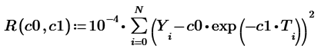
(T, Y) is an array of N experimental points, and we entered the multiplier for convenience (it does not affect the position of the minimum). Then, of course, you could immediately write one or two lines of code with a built-in minimum search function to get the desired C0 and C1, however, we use the free Mathcad Express, where they are all off, so let's go a little more cumbersome (but more easy to understand). and visual) by.
To begin with, let's see how the function R (c0, c1) behaves. To do this, we fix several values of c0 and construct for each of them a graph of the function of one variable R (c0, x).
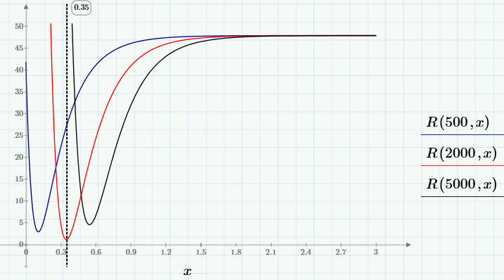
It can be seen that for selected c0, any of the graphs of the family has one minimum, whose position x depends on c0, i.e. you can write x = g (c0). The deepest minimum, i.e., the minimum of R (c0, g (c0)) ~ min, is the desired global minimum. We need to find it to solve the problem. To find the global minimum, first (using the means available in Mathcad Express) we define the user function g (y), and then find the minimum R (y, g (y)).
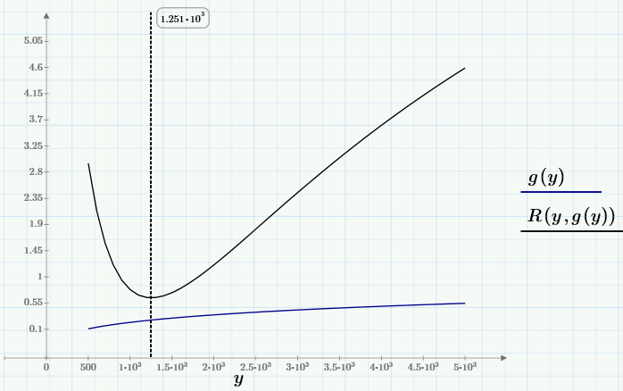
I will not dwell on the numerical algorithm for calculating the minimum (who cares, it is given in the first line of the next screenshot). The solution of the problem (a point, in the chosen notation c0 = y0 and c1 = x0), the value of the objective function at this point and the regression graph are given below:
Can we satisfy the result? Rather, no, since the constructed regression does not fit well with the experimental points. The “tail” interferes, which is very different for the regression (the exponent quickly drops to almost zero) and data (as you can see, even after a considerable time, the number of views is non-zero, and amounts to about a hundred).
Therefore, to improve the result, let's improve the model. We will consider the model of the number of article views as the sum of visits going through two channels:
This third parameter c2 can just be determined from the analysis of the “tail” of data, when there are practically no Poisson visitors, simply as the average value of views over the last 10 days of observations.
Finally, knowing c2, we can construct a refined regression of the form
Views ≈ c0 ∙ exp (c1 ∙ t) + c2,
completely repeating the algorithm described above:
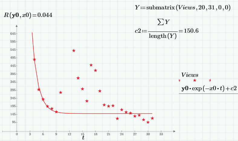
Please note that the value of the objective function at the minimum (i.e. the sum of squared residuals) decreases as compared with the case c2 = 0 more than an order of magnitude!
In conclusion, I’ll give the result of the built-in expfit function for finding the exponential regression (available in the commercial version of Mathcad Prime). The result of the work is shown on the graph in green dotted line, and our result (the same as in the previous graph) is shown in red solid line.
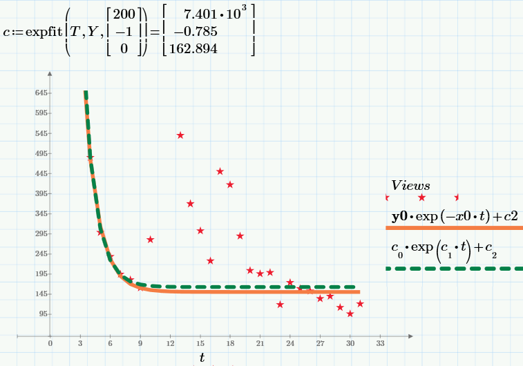
All pictures are screenshots of Mathcad Express (you can take the calculations here, repeat them, and if you want to change them and use them for your needs). Do not forget to set c2 = 0 or c2 = 150 at the beginning of the calculations to select the first or second model, respectively.
When it is known that the random variable y depends on something (for example, on time or on another random variable x) linearly, i.e. According to the law y (x) = Ax + b, linear regression is applied (as in the previous article, we built the dependence of the number of registrations on the number of views). For linear regression, the coefficients A and b are calculated using the known formulas. In the case of another type of regression, for example, exponential, in order to determine the unknown parameters, it is necessary to solve the corresponding optimization problem: namely, in the framework of the least squares method (OLS), the problem of finding the minimum of the sum of squares (y (x i ) - y i ) 2 .
So, here are the data that we will use as an example. Attendance peaks (Views row, red dotted line) are at the time of publication of articles. The second data series (Regs, with a multiplier of 100) shows the number of readers who performed a certain action after reading (registering and downloading Mathcad Express - with its help, by the way, you can repeat all the calculations of this and previous articles). All the pictures are screenshots of Mathcad Express, and you can take the file with the calculations here .
')
With the green arrow on the graph, I have designated the data fragment for which we will build a non-linear regression. According to the model that we take as the basis, after a short transition period after the publication, the number of views decreases with time approximately exponentially:
Views ≈ C 0 ∙ exp (C 1 ∙ t).
The justification of this model will be postponed until one of the future articles, when it comes to the Poisson random process.
It is clear that for the analysis it is necessary to select the fragment that corresponds to the model (not too close to the initial peak and without summation with the statistics of visits after the second article was released). This interval is highlighted by the green arrow on the first graph, and on a larger scale it looks like this:
The exponential regression, I recall, will determine the graph of such an exponential function that will be “on average” closest to the experimental points shown. In order to find the regression coefficients, it will be necessary to solve an optimization problem for finding the minimum of the objective function:
(T, Y) is an array of N experimental points, and we entered the multiplier for convenience (it does not affect the position of the minimum). Then, of course, you could immediately write one or two lines of code with a built-in minimum search function to get the desired C0 and C1, however, we use the free Mathcad Express, where they are all off, so let's go a little more cumbersome (but more easy to understand). and visual) by.
To begin with, let's see how the function R (c0, c1) behaves. To do this, we fix several values of c0 and construct for each of them a graph of the function of one variable R (c0, x).
It can be seen that for selected c0, any of the graphs of the family has one minimum, whose position x depends on c0, i.e. you can write x = g (c0). The deepest minimum, i.e., the minimum of R (c0, g (c0)) ~ min, is the desired global minimum. We need to find it to solve the problem. To find the global minimum, first (using the means available in Mathcad Express) we define the user function g (y), and then find the minimum R (y, g (y)).
I will not dwell on the numerical algorithm for calculating the minimum (who cares, it is given in the first line of the next screenshot). The solution of the problem (a point, in the chosen notation c0 = y0 and c1 = x0), the value of the objective function at this point and the regression graph are given below:
Can we satisfy the result? Rather, no, since the constructed regression does not fit well with the experimental points. The “tail” interferes, which is very different for the regression (the exponent quickly drops to almost zero) and data (as you can see, even after a considerable time, the number of views is non-zero, and amounts to about a hundred).
Therefore, to improve the result, let's improve the model. We will consider the model of the number of article views as the sum of visits going through two channels:
- channel with Poisson statistics Views ≈ c0 ∙ exp (c1 ∙ t);
- channel with approximately constant number of views (let's call it the parameter c2).
This third parameter c2 can just be determined from the analysis of the “tail” of data, when there are practically no Poisson visitors, simply as the average value of views over the last 10 days of observations.
Finally, knowing c2, we can construct a refined regression of the form
Views ≈ c0 ∙ exp (c1 ∙ t) + c2,
completely repeating the algorithm described above:
Please note that the value of the objective function at the minimum (i.e. the sum of squared residuals) decreases as compared with the case c2 = 0 more than an order of magnitude!
In conclusion, I’ll give the result of the built-in expfit function for finding the exponential regression (available in the commercial version of Mathcad Prime). The result of the work is shown on the graph in green dotted line, and our result (the same as in the previous graph) is shown in red solid line.
All pictures are screenshots of Mathcad Express (you can take the calculations here, repeat them, and if you want to change them and use them for your needs). Do not forget to set c2 = 0 or c2 = 150 at the beginning of the calculations to select the first or second model, respectively.
Source: https://habr.com/ru/post/252571/
All Articles