DICOM Viewer from the inside. Voxel render
Good afternoon, dear Habra community!
Today I would like to shed light on one of the most unlighted topics on Habré. It will be about the medical radiological imaging visualizer or the DICOM Viewer. It is planned to write several articles in which we will talk about the main features of the DICOM Viewer, including the possibilities of the voxel render, 3D, 4D, consider its device, support for the DICOM protocol, etc. In this article I will talk about the voxel renderer and its device. All interested welcome under cat.
The company in which I work has extensive experience in the development of medical software. I had a chance to work with some projects, so I wanted to share my accumulated experience in this area and show what we did. I would also like to take this opportunity to get feedback from radiologists on the use of the Viewer.
')
One of our products is DICOM Viewer, a DICOM format medical image viewer. It can render 2D images, build 3D models based on 2D slices, and also supports operations for both 2D images and 3D models. I will write about Viewer's operations and capabilities in the next article. At the end of the article there will be links to the DICOM Viewer itself with full functionality, which is described in the article and to data for samples. But everything is in order.
To imagine how to build a 3D model, for example, of the brain, from 2D DICOM files, you need to understand how images are represented in medicine. To begin with, all modern tomographs (MRI, CT, PET) do not produce ready-made images. Instead, a file is created in a special DICOM format, which contains information about the patient, the study, as well as information for drawing the image. In fact, each file represents a slice of an arbitrary part of the body, in a plane, most often in a horizontal one. So each such DICOM file contains information about the intensity or density of tissues in a particular slice, on the basis of which the final image is built. In fact, intensity and density are different concepts. Computed tomography saves files x-ray density, which depends on the physical density of tissues. Bones have greater physical density, less blood, etc. A magnetic resonance tomograph retains the intensity of the reverse signal. We will use the term density, thus summarizing the concepts described above.
The density information in a DICOM file can be represented as a regular image, which has resolution, pixel size, format, and other data. Only instead of information about the color in the pixel stored information about the density of tissues.
The diagnostic station produces not one file, but several at once for one study. These files have a logical structure. Files are combined in a series and represent a set of consecutive sections of an organ. Series unite in stages. The stage defines the entire study. The sequence of the series in the stage is determined by the study protocol.
Information about the density of tissues in the DICOM file is the basis for its drawing. To draw an image, you need to match the density values with a color. This makes the transfer function, which can be edited in our viewer. In addition, there are many ready-made presets for drawing different density fabrics with different colors. Here is an example of the transfer function and the result of the drawing:

The graph shows two white dots at the ends of the white line, which means that only the white color will be drawn. The line connecting the dots means opacity, i.e. less dense fabrics are rendered with more transparent pixels. Thus, the white color plus the corresponding opacity value gives a gradation of white, which is evident in the picture. This example shows the relative transfer function, so the percentages are plotted on the abscissa. The blue color on the graph shows the density distribution of tissues, where each density value corresponds to the number of pixels (voxels) per given density.
In our render there is a drawing of white color with the corresponding transparency on a black background, the black color is never drawn. Such a scheme is convenient when rendering a 3D model - the air has a small density, therefore it is drawn transparent, so when overlaying slices through the air of the superimposed image, the bottom one will be visible. In addition, if the color had not a constant characteristic, but a linear one (what characterizes the transition from black to white), then multiplying the color by the transparency (which also has a linear characteristic) would result in a quadratic characteristic that would reflect the color otherwise, is not true.
Transfer functions are divided by type into absolute and relative. The absolute transfer function is constructed for all possible densities. For CT, this is the Hounsfield scale (from -1000 to ~ 3000). A density of -1000 corresponds to air, a density of 400 corresponds to bones, zero density corresponds to water. For densities on the Hounsfield scale, the following statement is true: each density corresponds to a particular type of tissue. However, this statement is not true for MRI, as the MRI for each series generates its own set of densities. That is, for two series the same density can correspond to different tissues of the body. In the absolute transfer function, the arguments correspond to the absolute values of the density.
The relative transfer function is built on the basis of the so-called window, which indicates exactly which density range to draw. The window is determined by the Window Width (W) and Window Center (L) parameters, the recommended values of which are set by the tomograph and stored in snapshot files in the corresponding DICOM tags. The values of W and L can be changed at any time. Thus, the window restricts the domain of the transfer function. In the relative transfer function, the arguments correspond to the relative values given in percentages. An example of the transfer function is shown in the figure above with a scale in percent from 0 to 100.
As in the case of the absolute and in the case of the relative transfer function, there are cases when the transfer function does not cover all the densities contained in the snapshot file. In this case, all the densities that fall to the right of the transfer function take the values of the rightmost value of the transfer function, and the densities on the left, the values of the leftmost value of the transfer function, respectively.
An example of an absolute transfer function in which the density is given in absolute values on the Hounsfield scale:
Here is an example of a more complex linear transfer function, which paints the density in several colors:

As in the previous figure, transparency has a linear characteristic. However, colors are specified for specific densities. In addition to color, each of these points defines transparency (according to the white line on the graph). In the case of a 3D model, each of the points also stores reflective components. Interpolation is performed between specific points for specific components, including transparency, RGB, reflective components, thus obtaining values for the remaining densities.
The transparency in the transfer function need not be linear. She can be of any order. An example of a transfer function with arbitrary transparency:

Among other things, on each 2D-image information about the image is drawn. In the lower right corner, an orientation cube is drawn, by which one can understand how the patient is located in this image. H - head (head), F - foot (legs), A - anterior (full face), P - posterior (back), L - left (left side), R - right (right side). The same letters are duplicated in the middle of each side. In the lower left and upper right corners for radiologists, information about the tomograph parameters with which this image was obtained is displayed. Also on the right is drawn a ruler and a scale of one division, respectively.
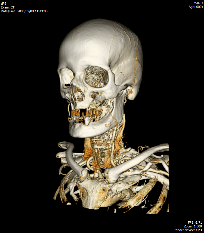
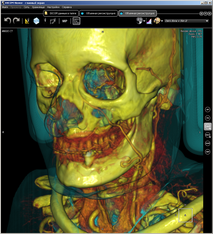
Since the voxel render is the basis for several of our projects, it is presented as a separate library. It is called VVL (ang. Volume Visualization Library). It is written in pure C without using any third-party libraries. VVL is designed for rendering three-dimensional models built from data from DICOM scanners (MRI, CT, PET). VVL uses all the advantages of modern multi-core processors for realtime rendering, so it can run on a conventional machine, and also has an implementation on CUDA, which gives a much higher performance than on a CPU. Here are a couple of images taken by the renderer based on computed tomography data.

VVL implements the entire drawing process, starting with building a model and ending with generating a 2D image. There are such features as resampling, anti-aliasing, translucency.
A voxel is an element of a three-dimensional image containing the value of an element in three-dimensional space. In general, anything can be a voxel value, including color. In our case, the density represents the value of the voxel. As for the shape of the voxel, in general, voxels can be cubic, or can be a parallelepiped. We have voxels in the form of cubes for simplicity and ease of operation. The coordinates of the voxels are not stored, they are calculated from the relative location of the voxel.
In fact, a voxel is a complete analogue of a pixel in 3D. Pixel (English picture element) - an element of the image, Voxel (English volume element) - a volume element. Almost all the characteristics of the pixel are transferred to the voxel, so you can safely draw analogies, given the dimension. Thus, voxels are used to represent three-dimensional objects:

In the screenshot you can see the small cubic voxels. A 2x byte number is used to store density in a voxel. Therefore, it is possible to calculate the size of the model: 2 bytes per density * number of voxels. Some voxel renders, in addition to the above, store information in the voxel for rendering, which requires additional memory. Practically we have established that it is inexpedient and it is more profitable to calculate the necessary data “on the fly” than to store extra bytes.
The input for the voxel render is the DICOM series, i.e. several images representing any area of the body. If images of one series are superimposed on each other in the sequence and in the plane in which they were made, a 3D model can be obtained. You can imagine this as something like this:

Since the DICOM protocol does not clearly declare in which tag the value of the distance between images in the series is stored, it is necessary to calculate the distance between images using other data. So, each image has space coordinates and orientation. This data is sufficient to determine the distance between the images. Thus, having the resolution of the image and the distance between them in a series, you can determine the size of the voxel. Image resolution in X and Y, as a rule, is the same, i.e. The pixel is square. But the distance between the images may differ from this value. Therefore, the voxel may be in the form of an arbitrary parallelepiped.
For ease of implementation and ease of operation, we do resampling for density values using bicubic filtering (Mitchell filter), and we get a cubic voxel shape. If the pixel size is smaller than the distance between the slices, we add supersampling slices, and if the pixel size is larger, then we remove the slices (downsampling). Thus, the pixel size becomes equal to the distance between the slices and we can build a 3D model with a cubic voxel shape. Simply put, we adjust the distance between the images to the image resolution.
Received voxels are stored in a structure representing an array optimized for access in an arbitrary direction of motion, in the case of drawing on the processor. The array is logically divided into parallelepipeds stored in memory in a continuous piece of ~ 1.5 kb in size with a voxel size of 2 bytes, which allows you to put several closely spaced parallelepipeds into the cache of the first level processor. Each parallelepiped stores 5x9x17 voxels. Based on the size of such a parallelepiped, the coordinates of the displacements in the general array of voxels are calculated and stored in 3 separate arrays xOffset, yOffset, zOffset. Therefore, the array is accessed as follows: m [xOffest [x] + yOffset [y] + zOffset [z]]. Thus, starting to read data in the parallelepiped, we force the processor to put the entire parallelepiped into the cache of the first level processor, which speeds up the data access time.
In the case of rendering on a GPU, a special three-dimensional structure is used in the graphics memory of the video card, called a 3D texture, the access to voxels in which is optimized by means of a video adapter.
Raytracing - as a way of rendering. Moving along the ray with some step and looking for the intersection with the voxel, and at each step we perform a trilinear interpolation, where 8 vertices represent the midpoints of the neighboring voxels. On the CPU, an octo tree is used as the optimal structure for quickly skipping transparent voxels. On a GPU for a 3D texture, trilinear interpolation is performed automatically by means of a video card. On the GPU, an octo-tree is not used to skip transparent pixels, because in the case of a 3D texture, it sometimes turns out that it is faster to take into account all voxels than to waste time searching and skipping transparent ones.
As the lighting model, Phong shading is used, which allows you to make an image volumetric and gives a good picture and at the same time does not interfere with the work of dentists. Raytracing is performed taking into account the transparency of voxels, which allows rendering translucent fabrics.
Render supports promising modes

and parallel projections

Perspective projection is more realistic. Moreover, it is necessary for virtual endoscopy, which I will discuss in the next article.
As promised links to DICOM Viewer and data for the test.
Today I would like to shed light on one of the most unlighted topics on Habré. It will be about the medical radiological imaging visualizer or the DICOM Viewer. It is planned to write several articles in which we will talk about the main features of the DICOM Viewer, including the possibilities of the voxel render, 3D, 4D, consider its device, support for the DICOM protocol, etc. In this article I will talk about the voxel renderer and its device. All interested welcome under cat.
The company in which I work has extensive experience in the development of medical software. I had a chance to work with some projects, so I wanted to share my accumulated experience in this area and show what we did. I would also like to take this opportunity to get feedback from radiologists on the use of the Viewer.
')
One of our products is DICOM Viewer, a DICOM format medical image viewer. It can render 2D images, build 3D models based on 2D slices, and also supports operations for both 2D images and 3D models. I will write about Viewer's operations and capabilities in the next article. At the end of the article there will be links to the DICOM Viewer itself with full functionality, which is described in the article and to data for samples. But everything is in order.
Representation of images in medicine
To imagine how to build a 3D model, for example, of the brain, from 2D DICOM files, you need to understand how images are represented in medicine. To begin with, all modern tomographs (MRI, CT, PET) do not produce ready-made images. Instead, a file is created in a special DICOM format, which contains information about the patient, the study, as well as information for drawing the image. In fact, each file represents a slice of an arbitrary part of the body, in a plane, most often in a horizontal one. So each such DICOM file contains information about the intensity or density of tissues in a particular slice, on the basis of which the final image is built. In fact, intensity and density are different concepts. Computed tomography saves files x-ray density, which depends on the physical density of tissues. Bones have greater physical density, less blood, etc. A magnetic resonance tomograph retains the intensity of the reverse signal. We will use the term density, thus summarizing the concepts described above.
The density information in a DICOM file can be represented as a regular image, which has resolution, pixel size, format, and other data. Only instead of information about the color in the pixel stored information about the density of tissues.
The diagnostic station produces not one file, but several at once for one study. These files have a logical structure. Files are combined in a series and represent a set of consecutive sections of an organ. Series unite in stages. The stage defines the entire study. The sequence of the series in the stage is determined by the study protocol.
2D render
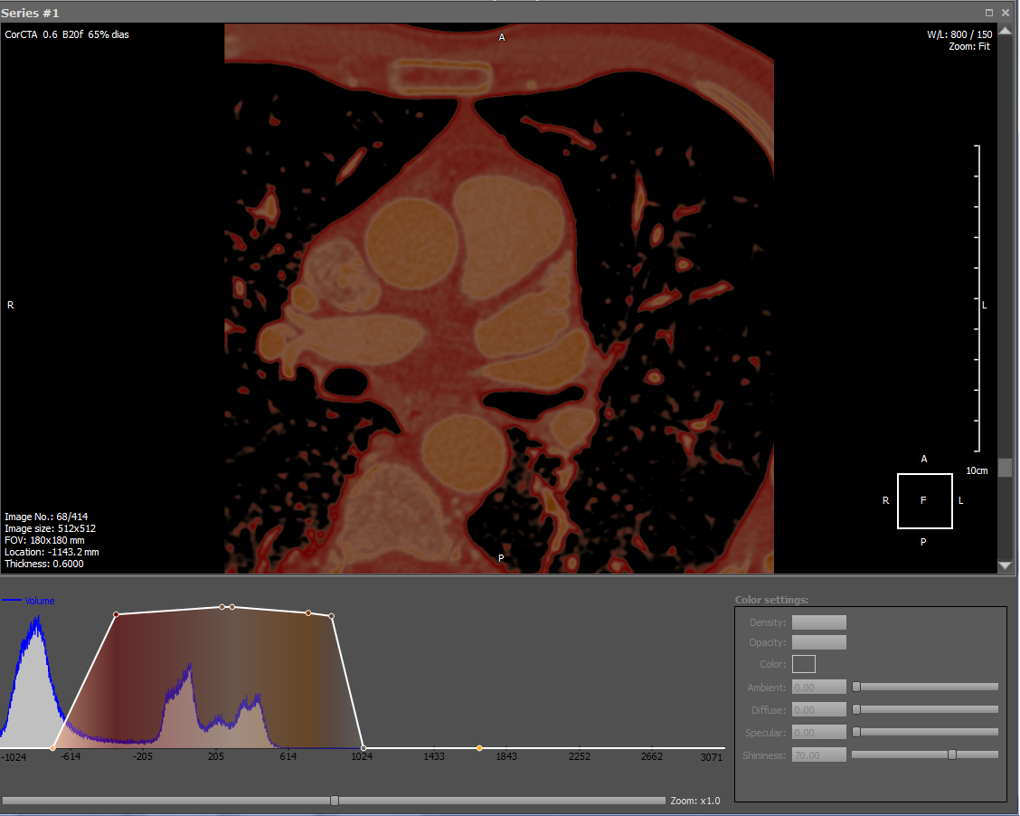
Information about the density of tissues in the DICOM file is the basis for its drawing. To draw an image, you need to match the density values with a color. This makes the transfer function, which can be edited in our viewer. In addition, there are many ready-made presets for drawing different density fabrics with different colors. Here is an example of the transfer function and the result of the drawing:
The graph shows two white dots at the ends of the white line, which means that only the white color will be drawn. The line connecting the dots means opacity, i.e. less dense fabrics are rendered with more transparent pixels. Thus, the white color plus the corresponding opacity value gives a gradation of white, which is evident in the picture. This example shows the relative transfer function, so the percentages are plotted on the abscissa. The blue color on the graph shows the density distribution of tissues, where each density value corresponds to the number of pixels (voxels) per given density.
In our render there is a drawing of white color with the corresponding transparency on a black background, the black color is never drawn. Such a scheme is convenient when rendering a 3D model - the air has a small density, therefore it is drawn transparent, so when overlaying slices through the air of the superimposed image, the bottom one will be visible. In addition, if the color had not a constant characteristic, but a linear one (what characterizes the transition from black to white), then multiplying the color by the transparency (which also has a linear characteristic) would result in a quadratic characteristic that would reflect the color otherwise, is not true.
Transfer functions are divided by type into absolute and relative. The absolute transfer function is constructed for all possible densities. For CT, this is the Hounsfield scale (from -1000 to ~ 3000). A density of -1000 corresponds to air, a density of 400 corresponds to bones, zero density corresponds to water. For densities on the Hounsfield scale, the following statement is true: each density corresponds to a particular type of tissue. However, this statement is not true for MRI, as the MRI for each series generates its own set of densities. That is, for two series the same density can correspond to different tissues of the body. In the absolute transfer function, the arguments correspond to the absolute values of the density.
The relative transfer function is built on the basis of the so-called window, which indicates exactly which density range to draw. The window is determined by the Window Width (W) and Window Center (L) parameters, the recommended values of which are set by the tomograph and stored in snapshot files in the corresponding DICOM tags. The values of W and L can be changed at any time. Thus, the window restricts the domain of the transfer function. In the relative transfer function, the arguments correspond to the relative values given in percentages. An example of the transfer function is shown in the figure above with a scale in percent from 0 to 100.
As in the case of the absolute and in the case of the relative transfer function, there are cases when the transfer function does not cover all the densities contained in the snapshot file. In this case, all the densities that fall to the right of the transfer function take the values of the rightmost value of the transfer function, and the densities on the left, the values of the leftmost value of the transfer function, respectively.
An example of an absolute transfer function in which the density is given in absolute values on the Hounsfield scale:
Here is an example of a more complex linear transfer function, which paints the density in several colors:
As in the previous figure, transparency has a linear characteristic. However, colors are specified for specific densities. In addition to color, each of these points defines transparency (according to the white line on the graph). In the case of a 3D model, each of the points also stores reflective components. Interpolation is performed between specific points for specific components, including transparency, RGB, reflective components, thus obtaining values for the remaining densities.
The transparency in the transfer function need not be linear. She can be of any order. An example of a transfer function with arbitrary transparency:
Among other things, on each 2D-image information about the image is drawn. In the lower right corner, an orientation cube is drawn, by which one can understand how the patient is located in this image. H - head (head), F - foot (legs), A - anterior (full face), P - posterior (back), L - left (left side), R - right (right side). The same letters are duplicated in the middle of each side. In the lower left and upper right corners for radiologists, information about the tomograph parameters with which this image was obtained is displayed. Also on the right is drawn a ruler and a scale of one division, respectively.
Voxel render
What is it ?
Since the voxel render is the basis for several of our projects, it is presented as a separate library. It is called VVL (ang. Volume Visualization Library). It is written in pure C without using any third-party libraries. VVL is designed for rendering three-dimensional models built from data from DICOM scanners (MRI, CT, PET). VVL uses all the advantages of modern multi-core processors for realtime rendering, so it can run on a conventional machine, and also has an implementation on CUDA, which gives a much higher performance than on a CPU. Here are a couple of images taken by the renderer based on computed tomography data.
VVL implements the entire drawing process, starting with building a model and ending with generating a 2D image. There are such features as resampling, anti-aliasing, translucency.
Inside voxel model
A voxel is an element of a three-dimensional image containing the value of an element in three-dimensional space. In general, anything can be a voxel value, including color. In our case, the density represents the value of the voxel. As for the shape of the voxel, in general, voxels can be cubic, or can be a parallelepiped. We have voxels in the form of cubes for simplicity and ease of operation. The coordinates of the voxels are not stored, they are calculated from the relative location of the voxel.
In fact, a voxel is a complete analogue of a pixel in 3D. Pixel (English picture element) - an element of the image, Voxel (English volume element) - a volume element. Almost all the characteristics of the pixel are transferred to the voxel, so you can safely draw analogies, given the dimension. Thus, voxels are used to represent three-dimensional objects:
In the screenshot you can see the small cubic voxels. A 2x byte number is used to store density in a voxel. Therefore, it is possible to calculate the size of the model: 2 bytes per density * number of voxels. Some voxel renders, in addition to the above, store information in the voxel for rendering, which requires additional memory. Practically we have established that it is inexpedient and it is more profitable to calculate the necessary data “on the fly” than to store extra bytes.
Model representation in memory
The input for the voxel render is the DICOM series, i.e. several images representing any area of the body. If images of one series are superimposed on each other in the sequence and in the plane in which they were made, a 3D model can be obtained. You can imagine this as something like this:
Since the DICOM protocol does not clearly declare in which tag the value of the distance between images in the series is stored, it is necessary to calculate the distance between images using other data. So, each image has space coordinates and orientation. This data is sufficient to determine the distance between the images. Thus, having the resolution of the image and the distance between them in a series, you can determine the size of the voxel. Image resolution in X and Y, as a rule, is the same, i.e. The pixel is square. But the distance between the images may differ from this value. Therefore, the voxel may be in the form of an arbitrary parallelepiped.
For ease of implementation and ease of operation, we do resampling for density values using bicubic filtering (Mitchell filter), and we get a cubic voxel shape. If the pixel size is smaller than the distance between the slices, we add supersampling slices, and if the pixel size is larger, then we remove the slices (downsampling). Thus, the pixel size becomes equal to the distance between the slices and we can build a 3D model with a cubic voxel shape. Simply put, we adjust the distance between the images to the image resolution.
Received voxels are stored in a structure representing an array optimized for access in an arbitrary direction of motion, in the case of drawing on the processor. The array is logically divided into parallelepipeds stored in memory in a continuous piece of ~ 1.5 kb in size with a voxel size of 2 bytes, which allows you to put several closely spaced parallelepipeds into the cache of the first level processor. Each parallelepiped stores 5x9x17 voxels. Based on the size of such a parallelepiped, the coordinates of the displacements in the general array of voxels are calculated and stored in 3 separate arrays xOffset, yOffset, zOffset. Therefore, the array is accessed as follows: m [xOffest [x] + yOffset [y] + zOffset [z]]. Thus, starting to read data in the parallelepiped, we force the processor to put the entire parallelepiped into the cache of the first level processor, which speeds up the data access time.
In the case of rendering on a GPU, a special three-dimensional structure is used in the graphics memory of the video card, called a 3D texture, the access to voxels in which is optimized by means of a video adapter.
Rendering
Raytracing - as a way of rendering. Moving along the ray with some step and looking for the intersection with the voxel, and at each step we perform a trilinear interpolation, where 8 vertices represent the midpoints of the neighboring voxels. On the CPU, an octo tree is used as the optimal structure for quickly skipping transparent voxels. On a GPU for a 3D texture, trilinear interpolation is performed automatically by means of a video card. On the GPU, an octo-tree is not used to skip transparent pixels, because in the case of a 3D texture, it sometimes turns out that it is faster to take into account all voxels than to waste time searching and skipping transparent ones.
As the lighting model, Phong shading is used, which allows you to make an image volumetric and gives a good picture and at the same time does not interfere with the work of dentists. Raytracing is performed taking into account the transparency of voxels, which allows rendering translucent fabrics.
Render supports promising modes
and parallel projections
Perspective projection is more realistic. Moreover, it is necessary for virtual endoscopy, which I will discuss in the next article.
As promised links to DICOM Viewer and data for the test.
Source: https://habr.com/ru/post/252429/
All Articles