We master technical vision on the example of Bioloid STEM and HaViMo2.0

Good afternoon, dear readers of Habr! With this article I open a series of publications on robotics. The main areas of focus of the articles will be the description of practical implementations of various tasks - from the simplest programming of robots to the implementation of navigation and autonomous behavior of the robot in various conditions. The main purpose of these articles is to show and teach how simple it is to solve a particular application task, or how to quickly adapt your robotic set to specific conditions. I will try to use the kits available and common in the market so that many of you can use my solutions and refine them for your own purposes. We hope that these articles will be useful both to students of various educational institutions and teachers of robotics.

Instead of the preface

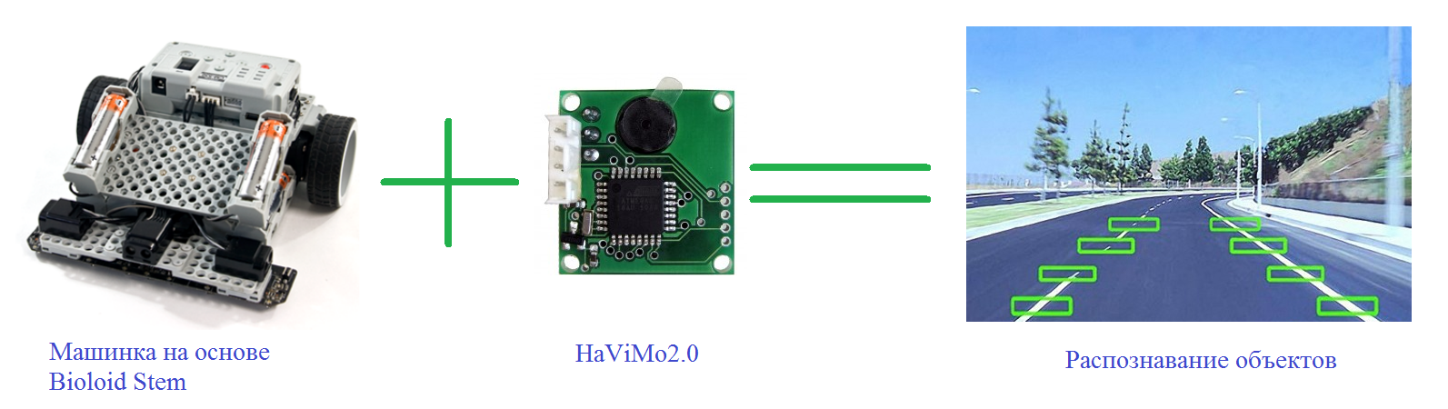
The work of modern mobile robots is often associated with constant and active movement in a dynamic (changeable) environment. Currently, due to the intensive robotization of the service sector, for example, the introduction of robokars in production, service robots for contact with people, there is a serious need to create such robots that could not only be able to move along predetermined routes and detect obstacles, but also to classify them in order to adapt flexibly to changing environments if necessary. This task can and should be solved using technical vision. In this paper, I propose to deal with the main points in the implementation of a technical vision using the example of using a machine from the Bioloid STEM robotic set and the HaViMo2.0 camera.
')
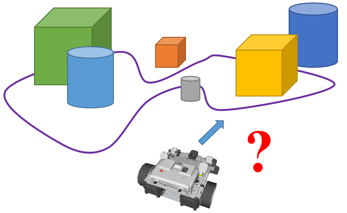
At present, such a movement of robots is widespread, as is driving along a line. This is widely used both at the factories in the AGV (Automatic Guided Vehicle) - robots move along pre-drawn lines, and when organizing robotic competitions - you can often meet tasks one way or another connected with orientation along lines. The main sensors with which the robot receives data are infrared sensors, which determine the difference in the contrast of the line and the ambient background, and magnetic sensors, which are used in the case of magnetic lines. The above examples of solutions require both thorough maintenance during operation and certain purity of the environment: for example, in a dirty warehouse, lines can get dirty and no longer recognized by IR sensors, and, for example, in metalworking magnetic lines can become clogged with iron chips. In addition to all this, it is assumed that the robot moves along predetermined routes, on which there should be no obstacles in the form of people whom it can cripple or in the form of any other objects. However, as a rule, there are always many moving objects in production that can potentially become an obstacle for the robot, so the robot should always not only receive information about its route and moving objects, but also have to analyze the environment so that, if necessary, be able to competently respond on the situation.


Figure 1. Warehouse robots moving along lines

When developing mobile robots, it is necessary to consider what tasks are set before the mobile robot in order to select the necessary sensor devices for their solution. For example, to solve the problem of moving within the working area, the robot can be equipped with expensive laser scanning range finders and GPS devices to determine its own position, while to solve the problem of local navigation, the mobile robot can be equipped with simple ultrasonic or infrared sensors around the perimeter. However, all the above means cannot give the robot a complete picture of what is happening around him, since the use of various distance sensors allows the robot to determine the distance to objects and their dimensions, but they do not allow to determine their other properties - shape, color, position in space, which leads to the impossibility to classify such objects by any criteria.



To solve the above problem, vision systems come to the rescue, allowing the robot to obtain the most complete information about the state of the environment around it. In essence, the technical vision system is the “eyes” of the robot, capable of using the camera to digitize the surrounding area and provide information about the physical characteristics of objects located in it in the form of data about
- sizes
- location in space
- appearance (color, surface condition, etc.)
- labeling (recognition of logos, barcodes, etc.).

The resulting data can be used to identify objects, measure their characteristics, as well as manage them.

The vision system is based on a digital camera that captures the surrounding space, then the data is processed by the processor using a specific image analysis algorithm to isolate and classify the parameters of interest to us. At this stage, the data are prepared and output in a form suitable for processing by the robot controller. Then the data is transmitted directly to the robot controller, where we can use it to control the robot.


Figure 2. The use of a vision system to monitor road conditions

As I mentioned earlier, our solution will be based on the popular robotic designer produced by Korean firm Robotis, namely the designer Bioloid STEM.


Figure 3. Constructor Bioloid STEM

This constructor contains components that allow you to assemble one of the 7 basic models of robots. I allow myself not to dwell on the detailed description of this set, since there are enough reviews of varying degrees of completeness on the network, for example, the Review of the designer Bioloid STEM . As a working model, we will use the standard set configuration - the Avoider machine.


Figure 4. Avoider is one of the 7 standard Bioloid STEM configurations

As the basis of the vision system, we will use the HaViMo2.0 image processing module, built on the basis of a color CMOS camera. This module is specifically designed for use with low-power processors. In addition to the camera, this module is equipped with a microcontroller that performs image processing, so the controller's resources for the image processing itself are not wasted. Data output is carried out through the serial port.


Figure 5. HaViMo2.0 image processing module


As you can see, HaViMo2.0 does not have official support for the CM-530 controller included in the Bioloid STEM kit. Nevertheless, it is possible to connect CM-530 and HaViMo2.0, but first things first.
First of all, we need to somehow install the image processing module on the typewriter. And the first thing that comes to mind is to fix the camera as shown on the models below. By the way, these models were obtained using the modeling environment from Bioloid - R + Design. This environment is “sharpened” especially for modeling robots from components offered by Bioloid. What is both good and bad at the same time. Since there is no image module in the R + Design parts collection, I have replaced it with a simulator with a similar-sized plate. And framed:


Figure 6. The location of the HaViMo2.0 image processing module on Avoider

Well, it should not look bad, but it is necessary to take into account another important point - the viewing angles of the camera module, because the image that the module will process will depend on it. Since the manufacturer HaViMo2.0 did not specify camera angles in the specification, I had to determine them myself. I do not pretend to high accuracy of determination, but the results I got are the following:

Viewing angles HaViMo2.0:
horizontal - 44 ° (no, I will not round up to 45 °, since I already rounded up to 44 °)
vertical - 30 °

I can say in advance - the results of the viewing angles correlated well with reality, so I will consider them as workers. Now, having the values ​​of viewing angles, I will formulate the task of locating the module as follows:

At what angle from the vertical it is necessary to reject the module at the location shown above in order to minimize the field of view, but at the same time exclude the elements of the robot from entering the field of view of the camera?

I decided to exactly minimize the scope for the following reasons:
- first, in practice, to check what comes of it
- secondly, to facilitate the subsequent calibration of the module for yourself (the less various objects fall within the scope, the easier it is to calibrate the module)

Let's draw our task on the plane (linear dimensions are indicated in mm, angular dimensions are in degrees):


Figure 7. Determining the angle of deviation of the module from the vertical

We know the position of the camera (C), we know the size of the front of the robot (AB), and we also know the vertical viewing angle (marked with red lines). Since there is nothing more complicated than the geometry of the 7th class, I allow myself not to lead the calculation (read - calculations) and say the answer immediately - there should be a 52 ° angle between the plane of the camera and the vertical (thanks to CAD for accuracy). When calculating manually, I got a value of 50 °, so we will consider the results acceptable.
In addition to the angle, we also obtained that the visible area of ​​the camera horizontally is about 85 mm.

The next step is to estimate how large the objects should be in order for them to be in the camera's field of view. We do this for the width of the line that the robot will have to track and move along it. Draw a drawing similar to the previous one for horizontal projection:


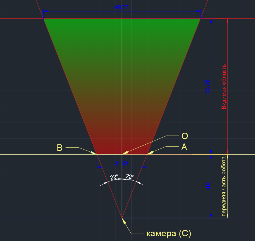
Figure 8. Visible area. Horizontal projection.

On this drawing, we again know the point of location of the camera (C), the size of the front of the robot (CO), the viewing angle horizontally, and we already know the length of the visible area, which we obtained in the previous step. Here we are primarily interested in the length of the segment AB, which shows the limiting value of the width of the object that the camera can fix. As a result, we have - if the robot goes along the line, then with this arrangement of the camera the line width should not exceed 31 mm. If the line is wider, we will not be able to accurately track its behavior.

Using the protractor and improvised means, I tried to fix the camera module as it was intended and this is what came of it:


Figure 9. Harsh reality - a living photo of the resulting structure

It's time to start working directly with the HaViMo2.0 module. Personally, I want to say from myself that this module is very capricious. Therefore, if something did not work for you, then try again. And better two.
Very important! The camera must be connected to the Dynamixel port located at the end of the controller between the battery connector and the Communication Jack.
To work with the camera and the subsequent programming of the robot, we need the following set of software:
- RoboPlus version 1.1.3.0 ( download from the manufacturer’s website )
- HaViMoGUI version 1.5 ( download )
- calibration firmware for CM-530 controller ( download )

Let's start with the preparation of the controller. Since the CM-530 controller bundled with the Bioloid STEM robotic kit is not officially supported by the image processing module, we need to use a custom firmware for the controller. So we reflash the controller. We connect the controller to the computer, turn it on with a toggle switch and perform the following actions:

1. Open RoboPlus
2. In the Expert tab, launch RoboPlus Terminal
3. We will see an error message, do not be alarmed and click OK. Note that No recent file is written in the lower left corner and Disconnect is written in the lower right corner:


Figure 10. Preparing the controller. Steps 1-3

4. Select the item Connect in the Setup menu. A window will appear with a choice of port and its setting. Select the COM port to which the controller is connected. Specify the speed - 57600. Click Connect. If the connection is successful, in the lower right corner Disconnect will change to the following: COM8-57600.
5. Without disconnecting the controller from the computer, turn it off with the POWER switch. Then we will make sure that we have the English keyboard layout set, hold down the Shift and 3 keys simultaneously (the three of them marked with #) and, without releasing the buttons, turn on the controller with a toggle switch. If everything is done correctly, system information will appear in the terminal window. Press Enter once.


Figure 11. Preparing the controller. Steps 4-5

6. Make sure that we have no wires hanging anywhere and the USB cable is securely connected to the computer and the controller. Further, it is forbidden to disconnect the controller from the PC and remove power from it. We will enter into the terminal the command l (English small L). Press Enter.
7. Select the menu item Transmit file. Select the downloaded custom firmware CM-530.hex and click the Open button.


Figure 12. Preparing the controller. Steps 6-7

8. After the download is complete, enter the GO command and press Enter. The terminal can be closed, the controller is disconnected from the computer.


Figure 13. Preparing the controller. Step 8

Our CM-530 controller is ready to work with the HaViMo2.0 module. Externally, it will not look very good - only one red LED will be lit, and it will not give any other signs of life. Do not be scared. This is normal. Now let's start calibrating our image processing module. Open HaViMoGUI, and the launch is carried out on behalf of the administrator. We will see the following window:


Figure 14. HaViMoGUI front panel

In the Connection Type item, select the CM-510 controller, in the Connection Port - the COM port number to which the controller is connected. Click Connect. In case of a successful connection, we will see Port Opened in the lower left corner of the window. Now connect directly to the camera. To do this, click Check Camera . If the connection to the camera was successful, then in the lower left corner we will see the inscription Check Camera: HaViMo2 Found. If such a label does not appear, check that the camera is connected to the controller correctly and repeat the steps starting from the launch of HaViMoGUI.


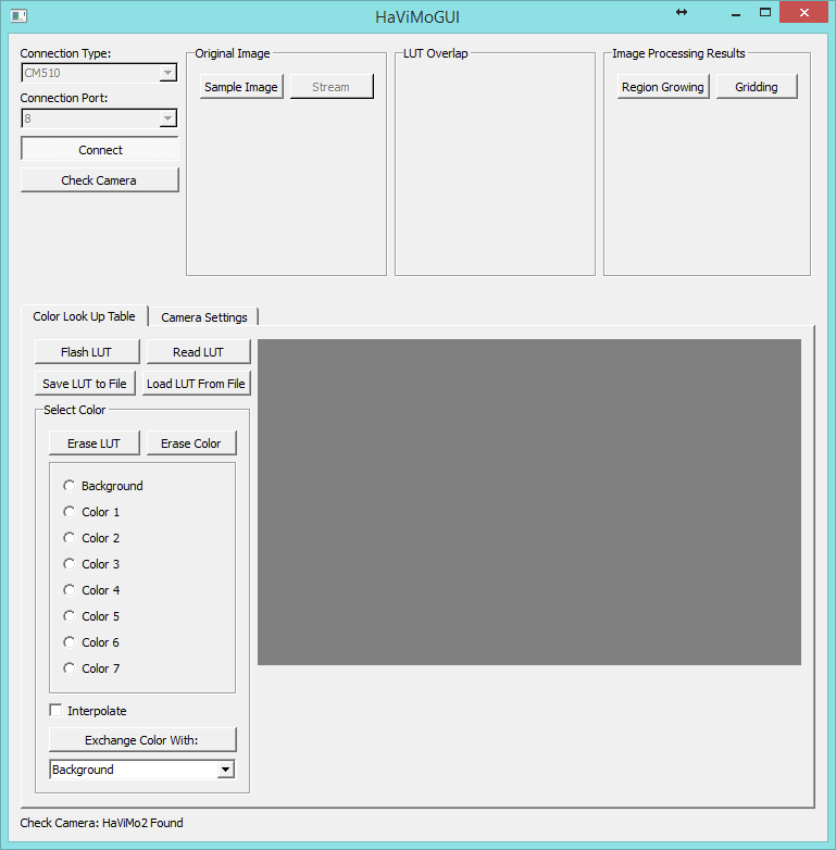
Figure 15. Camera connected successfully

Once connected to the camera, go to the Camera Settings tab and activate Auto Update Settings , which will allow the camera to automatically select the brightness / contrast (and other settings) of the image, depending on the brightness of the object.


Figure 16. Setting auto-settings

Then go back to the Color Look Up Table tab and click Sample Image to capture the image from the camera. As a result, we obtain an image of our object at the top of the window in the Original Image section. In the Color Look Up Table tab (right), the shades recognized by the camera appeared in the form of a 3D gradient. The camera recognizes an object by its color. At the same time, you can memorize 7 different objects (+ background). In order to memorize a color, in the Color Look Up Table tab, select Color 1 .


Figure 17. Capturing an image from a camera

You can select a color hue using a 3D gradient (click on the appropriate box) or by clicking on a specific Original Image point. In our case, we choose the white line, on which our robot will go. By clicking on Region Growing , we will see the recognition area that the module recognized. The simplest settings are made. In order to remember them, press the button Flash LUT . If the status bar says LUT Written Successfully, then the settings have been saved successfully. You can also save the settings to a separate file by clicking on the Save LUT to File button, to then read them from the file without first selecting the desired colors. The Read LUT button allows you to read the current camera settings.


Figure 18. Saving module settings

Setting up the image recognition module is solved. You can return the controller to the world of living and working controllers. To do this, launch RoboPlus, open the RoboPlus Manager and select the Controller Firmware Manager icon in the top line. Click Next .


Figure 19. Restoring controller firmware

Then we execute everything that the utility asks for us: in the window that appears, click on Find , then turn off and turn on the controller with the toggle switch. The controller should be detected by the utility, and then click Next twice.


Figure 20. Controller successfully detected

We are waiting for the installation of the firmware to finish, click Next , then Finish . After that, with a probability of 99%, we see an error that we don’t pay attention to - just close the window. This error occurs due to incorrect identification of the image recognition module connected to the controller. The controller is back in the living world - you can start programming it to control our robot.

We will develop the firmware in a standard environment from Robotis - RoboPlus Task. Programming in the RoboPlus Task is carried out using a specialized language similar to the C programming language. For the convenience of the user, RoboPlus implements the basic dialing capabilities in the form of graphic blocks, such as timers, data processing units from sensors, data transfer units between devices, etc. I will not dwell on the description of the programming process, as the environment is quite intuitive and does not cause difficulties. However, if you have any questions, I recommend to look at the development examples in the "Articles" and "Lessons" on our website . But before we start programming, let's look at how data is exchanged between the controller and the HaViMo2.0 module.

The connection between the module and the controller is implemented using the same protocol, which is used to exchange data between the controller and the Dynamixel AX-12 servos. The module itself is built around the DSP (Digital signal processor), which is configured through access to its registers, each of which can be read or configured using a calibration interface. A detailed description of the DSP settings is given in the manual modulo HaViMo2.0. There is also a complete list of registers. For us to work with the image processing module, it is enough to understand how data is output from the module.

The following example shows the output of the image processed by the module. Up to 15 areas with the address 0x10 to 0xFF can be read using the READ DATA (0x02) command. Each area consists of 16 bytes, which consist of the following parts:
- Region Index - Region Index: contains the value 0 if the region is not selected
- Region COLOR - Region Color
- Number of Pixels - Number of pixels: the number of detected pixels within the region.
- Sum of X Coordinates - Sum of Coordinates X: The result of adding the X coordinates of all detected points. Can be divided by the number of pixels to calculate the average X.
- Sum of Y Coordinates - The sum of Y coordinates: the result of adding the Y coordinates of all detected points. Can be divided by the number of pixels to calculate the average Y.
- Max X: Bounding side line to the right.
- Min X: Limiting side line to the right.
- Max Y: Limit line from below.
- Min Y: Limit line on top.


Figure 21. An example of image output from the HaViMo2.0 module

This example is enough to start programming the robot. In the RoboPlus Task environment, we write a function that will be responsible for determining the boundaries of the recognized area. Since this environment does not allow to display the code in a digestible text form, you will have to post screenshots. Let's call our function Get_Bounding_Box. The algorithm of the function is as follows:
- we sequentially poll the regions (Index) from 1 to 15 in a cycle, at each iteration of which we change the value of the address (Addr) in accordance with the rule specified above.
- if we find the recognized area (its index is not equal to 0), then we check it for compliance with the specified color (Color)
- if its color matches the specified one, we fix the size of the area (Size) and the values ​​of the bounding lines of our area (Maxx, Minx, Maxy, Miny)

Figure 22. Function code for determining the boundaries of the recognized area

Having obtained the values ​​of the size of the area and the coordinates of the bounding lines, you can proceed to programming the movement of the robot. The algorithm of the robot movement is quite simple, knowing the coordinates of the restrictive lines in X, we find the average X. When moving, if the average X is displaced, the robot will turn in the right direction, thereby self-positioning itself on the line along which it is traveling. Graphically, the algorithm for determining the movement of the robot is shown in the following figure:


Figure 23. Algorithm for determining the movement of the robot

And its text-block implementation:


Figure 24. Code of the main function of the program

So, to do this, when we turn on the controller, we first of all initialize our variables - the movement speeds, the forward movement time, the time during which the robot will perform the turn, and the time for pause. Further, in an infinite loop, we initialize the connection to the camera (specify the port number to which it is connected - CamID) and the color of the area, which we will detect. As we remember, during calibration we chose Color 1, so now we indicate it as interesting to us. After that, we turn to the camera and pause for 150 ms, because after the first call the camera does not respond for at least 128 ms. I put the function to initialize the camera connection in the main program loop, since the camera is very capricious and it may want to “fall off”. Initializing it at each iteration of the loop, we “ping” it, as it were. Then we call the function described above to determine the coordinates of the bounding lines of the recognized region and, based on the obtained values, we find the mean (Cx). And then we compare the obtained value for compliance with the conditions - if the obtained value is in a certain range, it means the robot goes straight, if it has shifted to the right - the robot turns it to the right, if it is to the left - accordingly to the left. The functions responsible for the movement are presented below:


Figure 25. Examples of functions that are responsible for moving forward and for turns to the left - to the right.

– , , . 2 :


26.

Everything. . , . :



, , , , . , . HaViMo2.0 :


27.

, , :


28.

, , , :


29. .

:


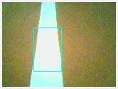
Figure 30. Interpretation of the recognition area in relation to our task.

Well, this is all great, but the camera does not allow us to transmit video in real time so that you can visually see what the camera sees and how it recognizes it. But I really wanted to track at least schematically what the camera recognizes, and how the robot behaves. For this, I used the LabView environment, with which I organized data collection from the CM-530 controller and its processing (For more information on how to collect data from the CM-530 controller, see my article “LabView in robotics - creating a SCADA system to control the robot”). Not that the utility turned out beautiful, but, in my opinion, quite useful for analyzing the movement of the robot. Since I did not have at hand any wireless adapter - neither ZigBee, nor Bluetooth, I had to drive data about the USB wire, which somewhat hampered my actions. The interface is as follows:


Figure 31. The interface of the application for analyzing the movement of the robot

And marking the recognition area, with explanations, in relation to our task:


32. ,

:
— : . , – . – , ( 29. – . – , , , – .
- the lower left window shows the position of the robot relative to the track in real time. Red lines, again, indicate the boundaries of our route, green dotted - middle.
- the lower right window shows the real movement of the robot - shooting the movement of the robot with a mobile phone camera.
- in the upper right, there are elements of the connection settings and indicators for displaying data from the robot, as well as a window for displaying an error if it occurs.
But it’s not interesting to look at the static picture, so I suggest you watch the video, where the whole process of the robot movement is clearly visible:



Now it is possible to analyze the movement of the robot in some detail. You can see the following things:
- the scope is reduced when the robot turns corners
- shadows (for example, from the wire) can interfere with recognition, again reducing the recognition area, so I highlighted for myself and want to offer you some recommendations that need to be considered when programming such a robot :

- “less is better, but more” - the lower the speed of movement and the less distance the robot travels per unit of time, the better, because the less likely the robot is to skip (“not see”) the turn, or leave the route badly;
- follows from the first recommendation - the sharper the angle of rotation, the greater the likelihood that the robot will miss it;
- our main enemy is floor covering. At this point, think for yourself what to do - I personally, for driving along linoleum, attached a sheet of paper to the lower part of the robot, since the resistance and creaking were terrible;
- Murphy's law - if a robot travels along a light line against a dark background and there is an object in the neighborhood that can be called light - know: for a robot, it will be the brightest, and he will gladly run to it;
- a consequence of the Murphy law - no matter how you reduce the camera's field of view, the robot will always find such a bright object;
- the robot can be afraid of its own shadow, so always think about how the light will fall, and train the recognition module to work in different lighting conditions;
- Be prepared for the fact that the batteries are discharged at the most inopportune moment, and outwardly it will look as if you have an error in the control program, the controller firmware, the controller itself and DNA. So always control the battery charge - for such a robot the normal voltage is 8-9V.

Well, in conclusion I would like to say that there is no limit to perfection - so everything is in your hands. Go ahead for adventures in the field of robotics!

Conclusion
Bioloid STEM – HaViMo2.0. . , , – , , – . , . See you again!