Lossy image compression
The idea behind all lossy compression algorithms is quite simple: in the first stage, delete irrelevant information, and in the second stage, apply the most appropriate lossless compression algorithm to the remaining data. The main difficulty lies in the allocation of this irrelevant information. The approaches here vary significantly depending on the type of compressible data. For sound, frequencies that a person is simply not able to perceive are most often removed, the sampling rate is reduced, and some algorithms remove quiet sounds immediately following loud ones, only moving objects are encoded for video data, and minor changes on fixed objects are simply discarded. Methods for extracting irrelevant information on images will be discussed in detail later.
Before talking about lossy compression algorithms, it is necessary to agree on what is considered acceptable loss. It is clear that the main criterion is the visual assessment of the image, but also changes in the compressed image can be quantified. The easiest way to estimate is to calculate the immediate difference between the compressed and original images. We agree that under we will understand the pixel located at the intersection of the i-th row and the j-th column of the original image, and by
  - the corresponding pixel of the compressed image. Then for any pixel you can easily determine the coding error
  , and for the entire image consisting of N rows and M columns, it is possible to calculate the total error
  . Obviously, the larger the total error, the greater the distortion in the compressed image. However, this value is extremely rarely used in practice, because It does not take into account the size of the image. Much more widely applied estimate using the standard deviation
 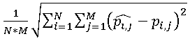 .
.
Another (albeit similar in essence) approach is as follows: the pixels of the final image are considered as the sum of the pixels of the original image and noise. The quality criterion for this approach is called the signal-to-noise ratio (SNR), calculated as follows: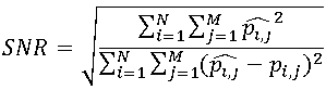 .
.
Both of these estimates are so-called. objective criteria of fidelity reproduction, because depend solely on the original and compressed image. However, these criteria do not always correspond to subjective assessments. If the images are intended for human perception, the only thing that can be argued is that poor indicators of objective criteria most often correspond to low subjective evaluations, while good indicators of objective criteria do not guarantee high subjective evaluations.
The concept of visual redundancy is associated with the quantization and discretization process. Much of the information in the image can not be perceived by man: for example, a person is able to notice slight differences in brightness, but is much less sensitive to chromaticity. Also, starting from a certain moment, increasing the sampling accuracy does not affect the visual perception of the image. Thus, some of the information can be deleted without compromising visual quality. This information is called visually redundant.
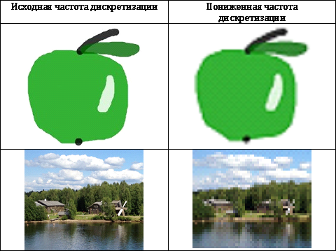
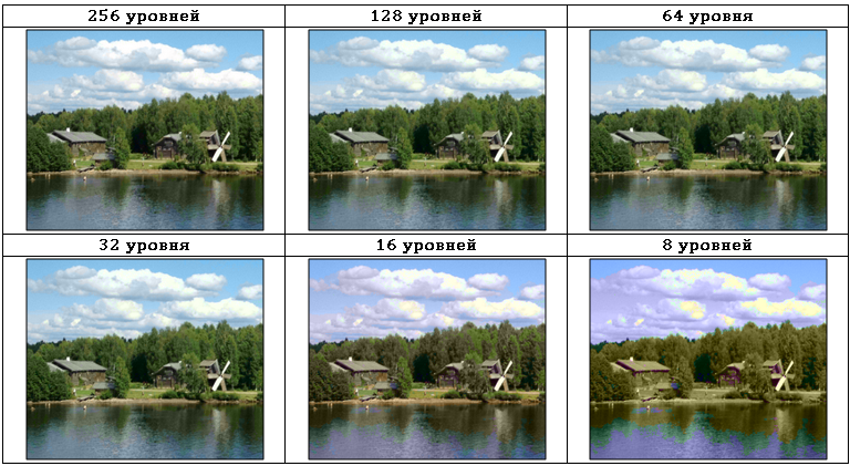
The easiest way to remove visual redundancy is to reduce the sampling accuracy, but in practice this method can only be used for images with a simple structure, because distortions that occur in complex images are too noticeable (see. Table 1)
')
To remove redundant information, quantization accuracy is often reduced, but it cannot be reduced thoughtlessly, since This leads to a sharp deterioration in image quality.
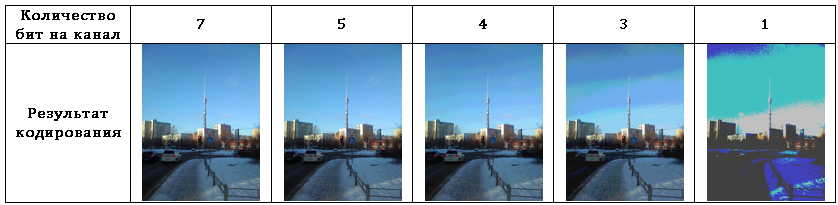
Consider the image already known to us with. Suppose that the image is represented in the RGB color space, the results of encoding this image with reduced quantization accuracy are presented in Table. 2
In the above example, uniform quantization is used as the easiest way, but if it is important to preserve color reproduction more accurately, you can use one of the following approaches: either use uniform quantization, but choose the mean of the segment, but the expected value of the segment, but use uneven splitting of the entire range of brightness.
Having carefully studied the obtained images, one can notice that on the compressed images there are distinct false contours, which significantly impair visual perception. There are methods based on transferring the quantization error to the next pixel, which can significantly reduce or even completely remove these contours, but they lead to image noise and graininess. These shortcomings severely limit the direct use of quantization for image compression.
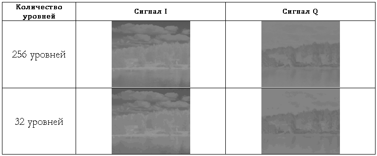
Most modern methods for removing visually abundant information use information about the features of human vision. Everyone knows the different sensitivity of the human eye to information about the color and brightness of the image. Tab. 3 shows an image in the YIQ color space, encoded with different quantization depth of the color difference signals IQ:
As can be seen from Tab. 3, the quantization depth of color difference signals can be lowered from 256 to 32 levels with minimal visual changes. At the same time, the losses in the I and Q components are very significant and are shown in Table. four
Despite the simplicity of the methods described, in their pure form they are rarely used, most often they serve as one of the steps of more efficient algorithms.
We have already considered predictive coding as a very efficient method of lossless data compression. If you combine coding with prediction and compression by quantization, you get a very simple and effective lossy image compression algorithm. In this method, the prediction error will be quantized. It is the accuracy of its quantization that will determine both the compression ratio and the distortions introduced into the compressed image. The choice of optimal algorithms for prediction and for quantization is a rather difficult task. In practice, the following universal (ensuring acceptable quality on most images) predictors are widely used:

We, in turn, take a detailed look at the simplest and at the same time very popular lossy coding method - the so-called. delta modulation. This algorithm uses prediction based on one previous pixel, i.e. . The error obtained after the prediction stage is quantized as follows:
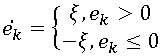
At first glance, this is a very crude method of quantization, but it has one indisputable advantage: the result of the prediction can be encoded with a single bit. Tab. Figure 5 shows images encoded with delta modulation (row-wrap) with different ξ values.
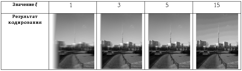
Two types of distortion are most noticeable - blurring of contours and a certain graininess of the image. This is the most typical distortion arising due to overload on the slope and because of the so-called. noise granularity. Such distortions are characteristic of all lossy coding variants with prediction, but using the example of delta modulation they are best seen.
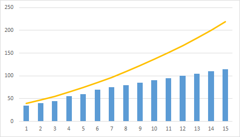
Noise of granularity arises mainly on monochromatic areas, when the value of ξ is too large to correctly display small fluctuations in brightness (or their absence). In Fig. 1, the yellow line indicates the original brightness, and the blue bars indicate the noise that occurs when quantizing the prediction error.

The situation of overload on a slope is fundamentally different from the situation with noise of granularity. In this case, the value of ξ is too small to transmit a sharp brightness difference. Due to the fact that the brightness of the encoded image can not grow as fast as the brightness of the original image, there is a noticeable blur of contours. The situation with overload on the slope is explained in Fig. 2
It is easy to see that the granularity noise decreases with decreasing ξ, but at the same time the distortions due to the overload due to the steepness grow and vice versa. This leads to the need to optimize the value of ξ. For most images, it is recommended to choose ξ∈ [5; 7].
All the previously discussed methods of image compression worked directly with the pixels of the original image. This approach is called spatial coding. In the current section, we consider a fundamentally different approach, called transformational coding.
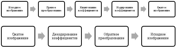
The basic idea of the approach is similar to the previously considered compression method using quantization, but it is not the brightness values of the pixels that will be quantized, but the conversion factors (transformations) calculated in a special way. Diagrams of transformational compression and image recovery are shown in Fig. 3, Fig. four.
Direct compression does not occur at the time of encoding, but at the time of quantizing the coefficients, since for most real-life images, most of the coefficients can be roughly quantized.
To obtain the coefficients, reversible linear transformations are used: for example, a Fourier transform, a discrete cosine transform, or a Walsh-Hadamard transform. The choice of a particular transformation depends on the permissible level of distortion and the resources available.
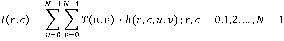
In the general case, an image with the dimensions N * N of pixels is considered as a discrete function of two arguments I (r, c), then the direct transformation can be expressed as follows:

Set just is the desired set of coefficients. Based on this set, you can restore the original image using the inverse transform:
Functions They are called transformation kernels, and the function g is the kernel of the direct transformation, and the function h is the kernel of the inverse transformation. The choice of transformation core determines both the compression efficiency and the computational resources required to perform the conversion.
Most often, transformational coding uses the kernels listed below.
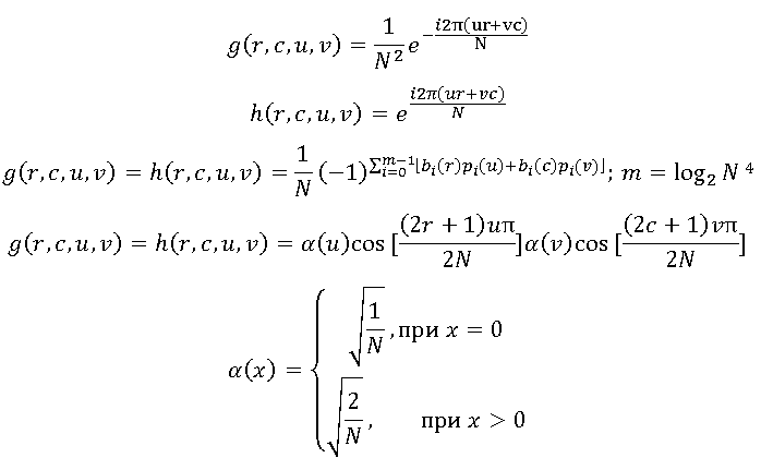
The use of the first two nuclei of these nuclei leads to a simplified version of the discrete Fourier transform. The second pair of cores corresponds to the often used Walsh-Hadamard transform. Finally, the most common transform is the discrete cosine transform:
The prevalence of discrete cosine transform is due to its good ability to compact the image energy. Strictly speaking, there are more efficient conversions. For example, the Karhunen-Loeve transformation has the best efficiency in terms of energy compaction, but its complexity practically excludes the possibility of wide practical application.
The combination of energy compression efficiency and comparative ease of implementation has made the discrete cosine transformation standard transformation coding.
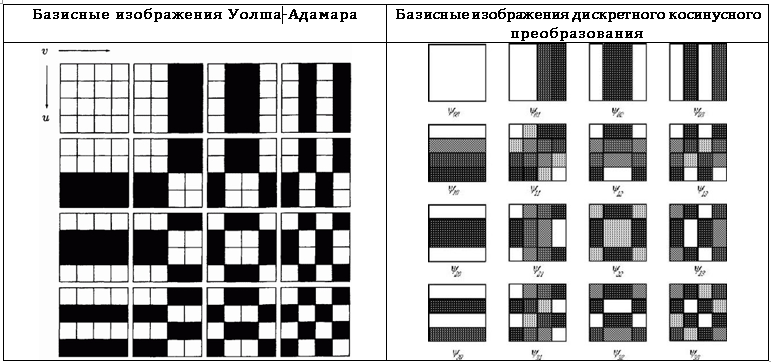
In the context of functional analysis, the considered transformations can be considered as an expansion over a set of basis functions. At the same time, in the context of image processing, these transformations can be perceived as decomposition into basis images. To clarify this idea, consider a square image I of size n * n pixels. The transformation cores do not depend on the transformation coefficients, nor on the pixel values of the original image, so the inverse transformation can be written in matrix form:

If these matrices are arranged in the form of a square, and the obtained values are presented in the form of pixels of a certain color, you can get a graphical representation of the basis functions, i.e. basic images. The basic images of the Walsh-Hadamard transform and the discrete cosine transform for n = 4 are given in Table. 7
The general idea of transformational coding was described earlier, but, nevertheless, the practical implementation of transformational coding requires clarification of several issues.
Before encoding the image is divided into square blocks, and then each block is subjected to conversion. Both the computational complexity and the final compression efficiency depend on the choice of the block size. As the block size increases, both compression efficiency and computational complexity increase, so in practice blocks of 8 * 8 or 16 * 16 pixels are most often used.
After the transformation coefficients are calculated for each block, it is necessary to quantize and encode them. The most common approaches are zonal and threshold coding.
In the zonal approach, it is assumed that the most informative coefficients will be located near the zero indices of the resulting array. This means that the corresponding coefficients must be most accurately quantized. Other coefficients can be quantized much rougher or simply discarded. The easiest way to understand the idea of zonal coding is by looking at the appropriate mask (Table 8):

The number in the cell indicates the number of bits reserved for encoding the corresponding coefficient.
Unlike zone coding, where the same mask is used for every block, threshold coding implies the use of a unique mask for each block. The threshold mask for the block is built on the basis of the following considerations: the most important factors for restoring the original image are the coefficients with the maximum value, therefore, keeping these coefficients and zeroing all the others, it is possible to provide both a high compression ratio and an acceptable quality of the reconstructed image. Tab. 9 shows an exemplary mask view for a specific block.

The units correspond to the coefficients that will be stored and quantized, and the zeros correspond to the coefficients that are thrown out. After applying the mask, the resulting matrix of coefficients must be converted into a one-dimensional array, and a snake bypass must be used for the conversion. Then, in the resulting one-dimensional array, all significant coefficients will be concentrated in the first half, and the second half will consist almost entirely of zeros. As was shown in earlier, such sequences are very efficiently compressed by run-length coding algorithms.
Wavelets - mathematical functions for analyzing the frequency components of data. In problems of information compression, wavelets are used relatively recently, however, researchers managed to achieve impressive results.
Unlike the transformations discussed above, wavelets do not require a preliminary splitting of the original image into blocks, but can be applied to the image as a whole. In this section, wavelet compression will be explained using a fairly simple Haar wavelet as an example.
First, consider the Haar transform for a one-dimensional signal. Let there be a set S of n values; in the Haar transformation, each pair of elements is assigned two numbers: the half-sum of the elements and their half-difference. It is important to note that this transformation is reversible: i.e. from a pair of numbers you can easily restore the original pair. In Fig. 5 shows an example of a one-dimensional Haar transform:

It can be seen that the signal is divided into two components: an approximate value of the original (with a resolution reduced by two times) and clarifying information.
The two-dimensional Haar transform is a simple composition of one-dimensional transforms. If the source data is presented in the form of a matrix, then a transformation is first performed for each row, and then a transformation is performed for the resulting matrices for each column. In Fig. 6 shows an example of a two-dimensional Haar transform.

The color is proportional to the value of the function at the point (the higher the value, the darker). As a result of the transformation, four matrices are obtained: one contains an approximation of the original image (with a reduced sampling frequency), and the other three contain clarifying information.
Compression is achieved by removing some of the coefficients from the refinement matrices. In Fig. 7 shows the recovery process and the reconstructed image itself after deleting from the refinement matrixes of coefficients of small modulus:

It is obvious that the representation of the image with the help of wavelets allows you to achieve effective compression, while maintaining the visual quality of the image. Despite its simplicity, the Haar transform is relatively rarely used in practice, since There are other wavelets that have several advantages (for example, Daubechay wavelets or biorthogonal wavelets).
PS Other chapters of the monograph are freely available on gorkoff.ru
Quality criteria for compressed images
Before talking about lossy compression algorithms, it is necessary to agree on what is considered acceptable loss. It is clear that the main criterion is the visual assessment of the image, but also changes in the compressed image can be quantified. The easiest way to estimate is to calculate the immediate difference between the compressed and original images. We agree that under
we will understand the pixel located at the intersection of the i-th row and the j-th column of the original image, and by - the corresponding pixel of the compressed image. Then for any pixel you can easily determine the coding error , and for the entire image consisting of N rows and M columns, it is possible to calculate the total error . Obviously, the larger the total error, the greater the distortion in the compressed image. However, this value is extremely rarely used in practice, because It does not take into account the size of the image. Much more widely applied estimate using the standard deviation .Another (albeit similar in essence) approach is as follows: the pixels of the final image are considered as the sum of the pixels of the original image and noise. The quality criterion for this approach is called the signal-to-noise ratio (SNR), calculated as follows:
.Both of these estimates are so-called. objective criteria of fidelity reproduction, because depend solely on the original and compressed image. However, these criteria do not always correspond to subjective assessments. If the images are intended for human perception, the only thing that can be argued is that poor indicators of objective criteria most often correspond to low subjective evaluations, while good indicators of objective criteria do not guarantee high subjective evaluations.
Compression through quantization and discretization
The concept of visual redundancy is associated with the quantization and discretization process. Much of the information in the image can not be perceived by man: for example, a person is able to notice slight differences in brightness, but is much less sensitive to chromaticity. Also, starting from a certain moment, increasing the sampling accuracy does not affect the visual perception of the image. Thus, some of the information can be deleted without compromising visual quality. This information is called visually redundant.
The easiest way to remove visual redundancy is to reduce the sampling accuracy, but in practice this method can only be used for images with a simple structure, because distortions that occur in complex images are too noticeable (see. Table 1)
')
To remove redundant information, quantization accuracy is often reduced, but it cannot be reduced thoughtlessly, since This leads to a sharp deterioration in image quality.
Consider the image already known to us with. Suppose that the image is represented in the RGB color space, the results of encoding this image with reduced quantization accuracy are presented in Table. 2
In the above example, uniform quantization is used as the easiest way, but if it is important to preserve color reproduction more accurately, you can use one of the following approaches: either use uniform quantization, but choose the mean of the segment, but the expected value of the segment, but use uneven splitting of the entire range of brightness.
Having carefully studied the obtained images, one can notice that on the compressed images there are distinct false contours, which significantly impair visual perception. There are methods based on transferring the quantization error to the next pixel, which can significantly reduce or even completely remove these contours, but they lead to image noise and graininess. These shortcomings severely limit the direct use of quantization for image compression.
Most modern methods for removing visually abundant information use information about the features of human vision. Everyone knows the different sensitivity of the human eye to information about the color and brightness of the image. Tab. 3 shows an image in the YIQ color space, encoded with different quantization depth of the color difference signals IQ:
As can be seen from Tab. 3, the quantization depth of color difference signals can be lowered from 256 to 32 levels with minimal visual changes. At the same time, the losses in the I and Q components are very significant and are shown in Table. four
Despite the simplicity of the methods described, in their pure form they are rarely used, most often they serve as one of the steps of more efficient algorithms.
Predictive coding
We have already considered predictive coding as a very efficient method of lossless data compression. If you combine coding with prediction and compression by quantization, you get a very simple and effective lossy image compression algorithm. In this method, the prediction error will be quantized. It is the accuracy of its quantization that will determine both the compression ratio and the distortions introduced into the compressed image. The choice of optimal algorithms for prediction and for quantization is a rather difficult task. In practice, the following universal (ensuring acceptable quality on most images) predictors are widely used:
We, in turn, take a detailed look at the simplest and at the same time very popular lossy coding method - the so-called. delta modulation. This algorithm uses prediction based on one previous pixel, i.e.
. The error obtained after the prediction stage is quantized as follows:At first glance, this is a very crude method of quantization, but it has one indisputable advantage: the result of the prediction can be encoded with a single bit. Tab. Figure 5 shows images encoded with delta modulation (row-wrap) with different ξ values.
Two types of distortion are most noticeable - blurring of contours and a certain graininess of the image. This is the most typical distortion arising due to overload on the slope and because of the so-called. noise granularity. Such distortions are characteristic of all lossy coding variants with prediction, but using the example of delta modulation they are best seen.
Noise of granularity arises mainly on monochromatic areas, when the value of ξ is too large to correctly display small fluctuations in brightness (or their absence). In Fig. 1, the yellow line indicates the original brightness, and the blue bars indicate the noise that occurs when quantizing the prediction error.
The situation of overload on a slope is fundamentally different from the situation with noise of granularity. In this case, the value of ξ is too small to transmit a sharp brightness difference. Due to the fact that the brightness of the encoded image can not grow as fast as the brightness of the original image, there is a noticeable blur of contours. The situation with overload on the slope is explained in Fig. 2
It is easy to see that the granularity noise decreases with decreasing ξ, but at the same time the distortions due to the overload due to the steepness grow and vice versa. This leads to the need to optimize the value of ξ. For most images, it is recommended to choose ξ∈ [5; 7].
Transformational coding
All the previously discussed methods of image compression worked directly with the pixels of the original image. This approach is called spatial coding. In the current section, we consider a fundamentally different approach, called transformational coding.
The basic idea of the approach is similar to the previously considered compression method using quantization, but it is not the brightness values of the pixels that will be quantized, but the conversion factors (transformations) calculated in a special way. Diagrams of transformational compression and image recovery are shown in Fig. 3, Fig. four.
Direct compression does not occur at the time of encoding, but at the time of quantizing the coefficients, since for most real-life images, most of the coefficients can be roughly quantized.
To obtain the coefficients, reversible linear transformations are used: for example, a Fourier transform, a discrete cosine transform, or a Walsh-Hadamard transform. The choice of a particular transformation depends on the permissible level of distortion and the resources available.
In the general case, an image with the dimensions N * N of pixels is considered as a discrete function of two arguments I (r, c), then the direct transformation can be expressed as follows:
Set
just is the desired set of coefficients. Based on this set, you can restore the original image using the inverse transform:Functions
They are called transformation kernels, and the function g is the kernel of the direct transformation, and the function h is the kernel of the inverse transformation. The choice of transformation core determines both the compression efficiency and the computational resources required to perform the conversion.Widespread transformation cores
Most often, transformational coding uses the kernels listed below.
The use of the first two nuclei of these nuclei leads to a simplified version of the discrete Fourier transform. The second pair of cores corresponds to the often used Walsh-Hadamard transform. Finally, the most common transform is the discrete cosine transform:
The prevalence of discrete cosine transform is due to its good ability to compact the image energy. Strictly speaking, there are more efficient conversions. For example, the Karhunen-Loeve transformation has the best efficiency in terms of energy compaction, but its complexity practically excludes the possibility of wide practical application.
The combination of energy compression efficiency and comparative ease of implementation has made the discrete cosine transformation standard transformation coding.
Graphic explanation of transformational coding
In the context of functional analysis, the considered transformations can be considered as an expansion over a set of basis functions. At the same time, in the context of image processing, these transformations can be perceived as decomposition into basis images. To clarify this idea, consider a square image I of size n * n pixels. The transformation cores do not depend on the transformation coefficients, nor on the pixel values of the original image, so the inverse transformation can be written in matrix form:
If these matrices are arranged in the form of a square, and the obtained values are presented in the form of pixels of a certain color, you can get a graphical representation of the basis functions, i.e. basic images. The basic images of the Walsh-Hadamard transform and the discrete cosine transform for n = 4 are given in Table. 7
Features of the practical implementation of transformational coding
The general idea of transformational coding was described earlier, but, nevertheless, the practical implementation of transformational coding requires clarification of several issues.
Before encoding the image is divided into square blocks, and then each block is subjected to conversion. Both the computational complexity and the final compression efficiency depend on the choice of the block size. As the block size increases, both compression efficiency and computational complexity increase, so in practice blocks of 8 * 8 or 16 * 16 pixels are most often used.
After the transformation coefficients are calculated for each block, it is necessary to quantize and encode them. The most common approaches are zonal and threshold coding.
In the zonal approach, it is assumed that the most informative coefficients will be located near the zero indices of the resulting array. This means that the corresponding coefficients must be most accurately quantized. Other coefficients can be quantized much rougher or simply discarded. The easiest way to understand the idea of zonal coding is by looking at the appropriate mask (Table 8):
The number in the cell indicates the number of bits reserved for encoding the corresponding coefficient.
Unlike zone coding, where the same mask is used for every block, threshold coding implies the use of a unique mask for each block. The threshold mask for the block is built on the basis of the following considerations: the most important factors for restoring the original image are the coefficients with the maximum value, therefore, keeping these coefficients and zeroing all the others, it is possible to provide both a high compression ratio and an acceptable quality of the reconstructed image. Tab. 9 shows an exemplary mask view for a specific block.
The units correspond to the coefficients that will be stored and quantized, and the zeros correspond to the coefficients that are thrown out. After applying the mask, the resulting matrix of coefficients must be converted into a one-dimensional array, and a snake bypass must be used for the conversion. Then, in the resulting one-dimensional array, all significant coefficients will be concentrated in the first half, and the second half will consist almost entirely of zeros. As was shown in earlier, such sequences are very efficiently compressed by run-length coding algorithms.
Wavelet compression
Wavelets - mathematical functions for analyzing the frequency components of data. In problems of information compression, wavelets are used relatively recently, however, researchers managed to achieve impressive results.
Unlike the transformations discussed above, wavelets do not require a preliminary splitting of the original image into blocks, but can be applied to the image as a whole. In this section, wavelet compression will be explained using a fairly simple Haar wavelet as an example.
First, consider the Haar transform for a one-dimensional signal. Let there be a set S of n values; in the Haar transformation, each pair of elements is assigned two numbers: the half-sum of the elements and their half-difference. It is important to note that this transformation is reversible: i.e. from a pair of numbers you can easily restore the original pair. In Fig. 5 shows an example of a one-dimensional Haar transform:
It can be seen that the signal is divided into two components: an approximate value of the original (with a resolution reduced by two times) and clarifying information.
The two-dimensional Haar transform is a simple composition of one-dimensional transforms. If the source data is presented in the form of a matrix, then a transformation is first performed for each row, and then a transformation is performed for the resulting matrices for each column. In Fig. 6 shows an example of a two-dimensional Haar transform.
The color is proportional to the value of the function at the point (the higher the value, the darker). As a result of the transformation, four matrices are obtained: one contains an approximation of the original image (with a reduced sampling frequency), and the other three contain clarifying information.
Compression is achieved by removing some of the coefficients from the refinement matrices. In Fig. 7 shows the recovery process and the reconstructed image itself after deleting from the refinement matrixes of coefficients of small modulus:
It is obvious that the representation of the image with the help of wavelets allows you to achieve effective compression, while maintaining the visual quality of the image. Despite its simplicity, the Haar transform is relatively rarely used in practice, since There are other wavelets that have several advantages (for example, Daubechay wavelets or biorthogonal wavelets).
PS Other chapters of the monograph are freely available on gorkoff.ru
Source: https://habr.com/ru/post/251417/
All Articles