Lossless Image Compression
As I promised earlier in the post , I present to you the second part of a large story about image compression. This time we will talk about lossless image compression methods.
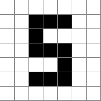
The easiest to understand algorithm is the series length coding algorithm developed in the 1950s. The main idea of the algorithm is to represent each line of a binary image as a sequence of lengths of continuous groups of black and white pixels. For example, the second line of the image shown in Fig. 1, will look like this: 2,3,2. But in the decoding process there will be ambiguity, since it is not clear which series: black or white encodes the first number. To solve this problem, there are two obvious methods: either for each row, preliminarily indicate the value of the first pixel, or agree that for each row, the length of the sequence of white pixels is first indicated (however, it may be zero).
The run-length coding method is very effective, especially for images with a simple structure, but this method can be significantly improved if the resulting sequences are additionally compressed by some entropy algorithm, for example, by the Huffman method. In addition, the entropy algorithm can be independently used separately for black and white sequences, which will further increase the compression ratio.
')
A further development of the idea of coding lengths of series is the compression method with tracing contours. This method is based on the use of high-level properties of the compressible image. Those. the image is perceived not just as a set of pixels, but as foreground objects and background. Compression is performed by efficiently representing objects. There are various ways of presenting, which we will look at next in the example of Pic. 2
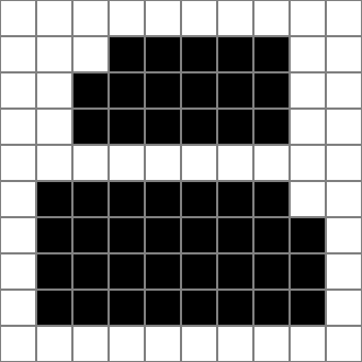
First of all, it should be noted that the description of each object should be enclosed in special messages (tags) of the beginning and end of the object. The first and easiest way is to specify the coordinates of the starting and ending point of the contour on each line. The image in Fig. 2 will be encoded as follows:
Of course, this record is further compressed using the previously discussed algorithms. But, again, the data can be converted in such a way as to increase the further degree of compression. For this, so-called. delta coding: instead of recording the immediate coordinates of the boundaries, their offset relative to the previous line is recorded. Using delta encoding, the image in Fig. 2 will be encoded as follows:
The efficiency of delta coding is explained by the fact that the magnitudes of the offsets in modulus are close to zero and with a large number of objects in their description there will be a lot of zero and close to zero values. The data thus transformed will be much better compressed by entropy algorithms.
Finishing the conversation about binary image compression, it is necessary to mention one more method - coding the domains of constancy. In this method, the image is divided into a rectangle of n 1 * n 2 pixels. All the resulting rectangles are divided into three groups: completely white, completely black and mixed. The most common category is encoded by a one-bit code word, and the remaining two categories receive codes of two bits. In this case, the code of the mixed area serves as a label, followed by n 1 * n 2 bits describing the rectangle. If you break the well-known image from Fig. 2 squares 2 * 2 pixels, you get five white squares, six black and 13 mixed. Let's agree 0 to designate a mixed square label, 11 - a white square label, and 10 - a black square label, a single white pixel will encode 1, and black, respectively, 0. Then the whole image will be encoded as follows (labels are highlighted in bold):

As with most compression methods, the effectiveness of this method is the higher, the larger the original image. In addition, you can see that the values of mixed squares can be very effectively compressed by dictionary algorithms.
This concludes the story of binary image compression and proceeds to the story of lossless compression of full-color and monochrome images.
There are many different approaches to lossless image compression. The most trivial are reduced to the direct application of the algorithms considered earlier in the post , other more advanced algorithms use information about the type of compressible data.
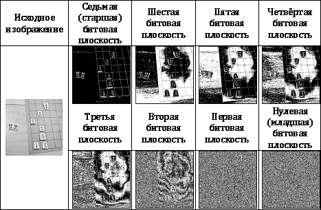
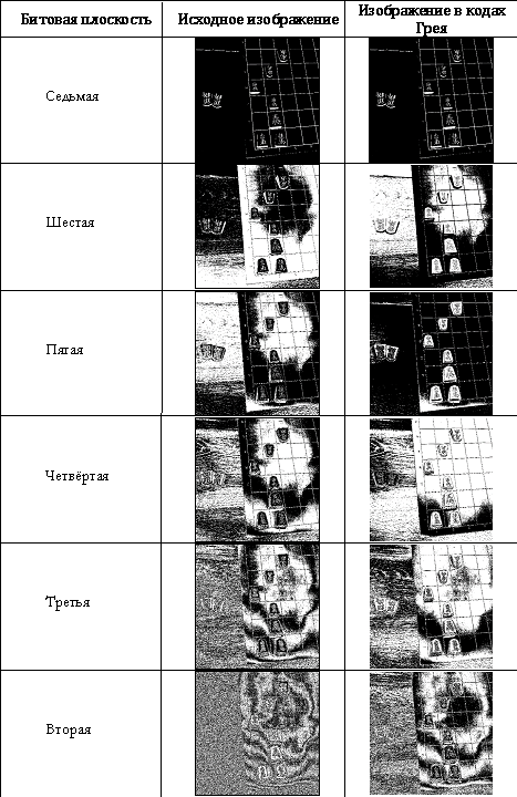
The first method that we consider will be a method known as encoding bit planes. Consider an arbitrary image with n brightness levels. Obviously, these levels can be represented using log 2 n bits. The method of decomposition into bit-planes consists in dividing one image with n levels of brightness into log 2 n binary images. In this case, the i-th image is obtained by extracting the i-th bits from each pixel of the original image. Tab. 1 shows the decomposition of the original image in bit planes.
After the image is decomposed into bit planes, each resulting image can be compressed using the binary image compression methods discussed earlier.
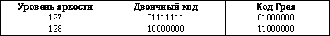
A rather obvious disadvantage of this approach is the effect of repeated transfer of discharges with a slight change in brightness. For example, when the brightness changes from 127 to 128, the values of all binary digits will change (0111111 → 10,000,000), which will cause a change in all bit planes.
In order to reduce the negative consequences of multiple hyphenation, in practice special codes are often used, for example, Gray codes, in which two neighboring elements differ only in one digit. To translate an n-bit number into a gray code, you must perform a bitwise exclusive OR operation with the same number shifted one bit to the right. The inverse transform from the gray code can be accomplished by performing a bitwise XOR operation for all shifts of the original number that are not equal to zero. Algorithms for converting to and from Gray code are shown in Listing 1.
It is easy to make sure that after converting to the Gray code, when changing the brightness from 127 to 128, only one binary bit changes:
The bit planes obtained using the Gray code are more monotonous and, in general, are better compressed. Tab. 2 shows the bit planes obtained from the original image, and the image converted to Gray code:
Predictive coding is based on an idea similar to the delta coding algorithm. Most real images are locally homogeneous, i.e. pixel neighbors have about the same brightness as the pixel itself. This condition is not satisfied on the borders of objects, but for most of the image it is true. Based on this, you can predict the brightness value of a pixel based on the brightness of its neighbors. Of course, this prediction will not be completely accurate, and a prediction error will occur. It is this prediction error that is further encoded using entropy algorithms. The coding efficiency is ensured by the already mentioned local homogeneity property: in most of the image, the magnitude of the error modulus will be close to zero.
With this encoding method, it is very important that the same predictor is used in both encoding and decoding. In the general case, the predictor can use any characteristics of the image, but in practice the predicted value is most often calculated as a linear combination of the brightness of the neighbors: p k = ∑ i = 1 M α i * p ki . In this formula, M is the number of neighbors involved in the prediction (the prediction order), the indices p are the numbers of the pixels in the order in which they are viewed. It can be noted that with M = 1, the predictive coding turns into the previously considered delta encoding (although instead of the difference in coordinates, the difference in brightness is now encoded).
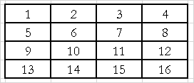
Here it is necessary to slightly discuss the order of viewing pixels. Up to this point, we assumed that the pixels are viewed from left to right and from top to bottom, i.e. in line bypass order (Table 3):
But it is obvious that the result of predicting the brightness of the fifth pixel on the basis of the fourth (when traversing by strings) will be very far from the true result. Therefore, in practice, other bypass orders are often used, for example, bypassing lines with reversal, snake, stripes, reversing stripes, etc. Some of the listed workarounds are listed in Table. four

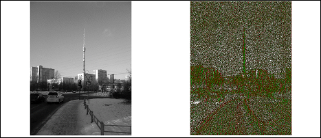
Consider the described method on a specific example. Let us try to apply prediction coding to the image of the Ostankino television tower in Fig. 3

For simplicity, we will use the first-order prediction (delta encoding) and crawling in rows (we will encode each line independently). In a software implementation, it is necessary to decide how to transmit information about the first M pixels whose value cannot be predicted. The implementation of Listing 2 uses the following approach: the first pixel of each row is encoded directly by its brightness value, and all subsequent pixels in the row are predicted based on the previous one.
Tab. 5 shows the result of this algorithm. Pixels predicted accurately are shown in white, and errors are marked in color, with a positive error value displayed in red and a negative value in green. The intensity of the color corresponds to the magnitude of the error.
Analysis shows that such an implementation provides an average prediction error of just 0.21 of the brightness level. The use of higher-order predictions and other workarounds makes it possible to further reduce the prediction error, and thus increase the degree of compression.
Binary Compression
Run length coding method
The easiest to understand algorithm is the series length coding algorithm developed in the 1950s. The main idea of the algorithm is to represent each line of a binary image as a sequence of lengths of continuous groups of black and white pixels. For example, the second line of the image shown in Fig. 1, will look like this: 2,3,2. But in the decoding process there will be ambiguity, since it is not clear which series: black or white encodes the first number. To solve this problem, there are two obvious methods: either for each row, preliminarily indicate the value of the first pixel, or agree that for each row, the length of the sequence of white pixels is first indicated (however, it may be zero).
The run-length coding method is very effective, especially for images with a simple structure, but this method can be significantly improved if the resulting sequences are additionally compressed by some entropy algorithm, for example, by the Huffman method. In addition, the entropy algorithm can be independently used separately for black and white sequences, which will further increase the compression ratio.
')
Contour coding method
A further development of the idea of coding lengths of series is the compression method with tracing contours. This method is based on the use of high-level properties of the compressible image. Those. the image is perceived not just as a set of pixels, but as foreground objects and background. Compression is performed by efficiently representing objects. There are various ways of presenting, which we will look at next in the example of Pic. 2
First of all, it should be noted that the description of each object should be enclosed in special messages (tags) of the beginning and end of the object. The first and easiest way is to specify the coordinates of the starting and ending point of the contour on each line. The image in Fig. 2 will be encoded as follows:
< START >
PAGE 2 4 - 8
PAGE 3 3 - 8
PAGE 4 3 - 8
< END >
< START >
PAGE 6 2 - 8
PAGE 7 2 - 9
PAGE 8 2 - 9
PAGE 9 2 - 9
< END >
Of course, this record is further compressed using the previously discussed algorithms. But, again, the data can be converted in such a way as to increase the further degree of compression. For this, so-called. delta coding: instead of recording the immediate coordinates of the boundaries, their offset relative to the previous line is recorded. Using delta encoding, the image in Fig. 2 will be encoded as follows:
< START >
PAGE 2 4 , 8
PAGE 3 - 1 , 0
PAGE 4 0 , 0
< END >
< START >
PAGE 6 2 , 8
PAGE 7 0 , 1
PAGE 8 0 , 0
PAGE 9 0 , 0
< END >
The efficiency of delta coding is explained by the fact that the magnitudes of the offsets in modulus are close to zero and with a large number of objects in their description there will be a lot of zero and close to zero values. The data thus transformed will be much better compressed by entropy algorithms.
Coding of persistence domains
Finishing the conversation about binary image compression, it is necessary to mention one more method - coding the domains of constancy. In this method, the image is divided into a rectangle of n 1 * n 2 pixels. All the resulting rectangles are divided into three groups: completely white, completely black and mixed. The most common category is encoded by a one-bit code word, and the remaining two categories receive codes of two bits. In this case, the code of the mixed area serves as a label, followed by n 1 * n 2 bits describing the rectangle. If you break the well-known image from Fig. 2 squares 2 * 2 pixels, you get five white squares, six black and 13 mixed. Let's agree 0 to designate a mixed square label, 11 - a white square label, and 10 - a black square label, a single white pixel will encode 1, and black, respectively, 0. Then the whole image will be encoded as follows (labels are highlighted in bold):
As with most compression methods, the effectiveness of this method is the higher, the larger the original image. In addition, you can see that the values of mixed squares can be very effectively compressed by dictionary algorithms.
This concludes the story of binary image compression and proceeds to the story of lossless compression of full-color and monochrome images.
Compress monochrome and full color images
There are many different approaches to lossless image compression. The most trivial are reduced to the direct application of the algorithms considered earlier in the post , other more advanced algorithms use information about the type of compressible data.
Bit Plane Coding
The first method that we consider will be a method known as encoding bit planes. Consider an arbitrary image with n brightness levels. Obviously, these levels can be represented using log 2 n bits. The method of decomposition into bit-planes consists in dividing one image with n levels of brightness into log 2 n binary images. In this case, the i-th image is obtained by extracting the i-th bits from each pixel of the original image. Tab. 1 shows the decomposition of the original image in bit planes.
After the image is decomposed into bit planes, each resulting image can be compressed using the binary image compression methods discussed earlier.
A rather obvious disadvantage of this approach is the effect of repeated transfer of discharges with a slight change in brightness. For example, when the brightness changes from 127 to 128, the values of all binary digits will change (0111111 → 10,000,000), which will cause a change in all bit planes.
In order to reduce the negative consequences of multiple hyphenation, in practice special codes are often used, for example, Gray codes, in which two neighboring elements differ only in one digit. To translate an n-bit number into a gray code, you must perform a bitwise exclusive OR operation with the same number shifted one bit to the right. The inverse transform from the gray code can be accomplished by performing a bitwise XOR operation for all shifts of the original number that are not equal to zero. Algorithms for converting to and from Gray code are shown in Listing 1.
function BinToGray ( BinValue : byte ) : byte ;
begin
BinToGray : = BinValue xor ( BinValue shr 1 ) ;
end ;
function GrayToBin ( GrayValue : byte ) : byte ;
var
BinValue : integer ;
begin
BinValue : = 0 ;
while GrayValue> 0 do
begin
BinValue : = BinValue xor GrayValue ;
GrayValue : = GrayValue shr 1 ;
end ;
GrayToBin : = BinValue ;
end ;
It is easy to make sure that after converting to the Gray code, when changing the brightness from 127 to 128, only one binary bit changes:
The bit planes obtained using the Gray code are more monotonous and, in general, are better compressed. Tab. 2 shows the bit planes obtained from the original image, and the image converted to Gray code:
Predictive coding
Predictive coding is based on an idea similar to the delta coding algorithm. Most real images are locally homogeneous, i.e. pixel neighbors have about the same brightness as the pixel itself. This condition is not satisfied on the borders of objects, but for most of the image it is true. Based on this, you can predict the brightness value of a pixel based on the brightness of its neighbors. Of course, this prediction will not be completely accurate, and a prediction error will occur. It is this prediction error that is further encoded using entropy algorithms. The coding efficiency is ensured by the already mentioned local homogeneity property: in most of the image, the magnitude of the error modulus will be close to zero.
With this encoding method, it is very important that the same predictor is used in both encoding and decoding. In the general case, the predictor can use any characteristics of the image, but in practice the predicted value is most often calculated as a linear combination of the brightness of the neighbors: p k = ∑ i = 1 M α i * p ki . In this formula, M is the number of neighbors involved in the prediction (the prediction order), the indices p are the numbers of the pixels in the order in which they are viewed. It can be noted that with M = 1, the predictive coding turns into the previously considered delta encoding (although instead of the difference in coordinates, the difference in brightness is now encoded).
Here it is necessary to slightly discuss the order of viewing pixels. Up to this point, we assumed that the pixels are viewed from left to right and from top to bottom, i.e. in line bypass order (Table 3):
But it is obvious that the result of predicting the brightness of the fifth pixel on the basis of the fourth (when traversing by strings) will be very far from the true result. Therefore, in practice, other bypass orders are often used, for example, bypassing lines with reversal, snake, stripes, reversing stripes, etc. Some of the listed workarounds are listed in Table. four
Consider the described method on a specific example. Let us try to apply prediction coding to the image of the Ostankino television tower in Fig. 3
For simplicity, we will use the first-order prediction (delta encoding) and crawling in rows (we will encode each line independently). In a software implementation, it is necessary to decide how to transmit information about the first M pixels whose value cannot be predicted. The implementation of Listing 2 uses the following approach: the first pixel of each row is encoded directly by its brightness value, and all subsequent pixels in the row are predicted based on the previous one.
type
TPredictionEncodedImg = array of array of integer ;
function DeltaEncoding : TPredictionEncodedImg ;
var
r : TPredictionEncodedImg ;
i , j : word ;
begin
SetLength ( r , GSI . N + 1 ) ;
for i : = 1 to GSI . N do
begin
SetLength ( r [ i ] , GSI . M + 1 ) ;
r [ i , 1 ] : = GSI . i [ i , 1 ] ;
end ;
for i : = 1 to GSI . N do
for j : = 2 to GSI . M do
r [ i , j ] : = GSI . i [ i , j ] - GSI . i [ i , j - 1 ] ;
DeltaEncoding : = r ;
end ;
Tab. 5 shows the result of this algorithm. Pixels predicted accurately are shown in white, and errors are marked in color, with a positive error value displayed in red and a negative value in green. The intensity of the color corresponds to the magnitude of the error.
Analysis shows that such an implementation provides an average prediction error of just 0.21 of the brightness level. The use of higher-order predictions and other workarounds makes it possible to further reduce the prediction error, and thus increase the degree of compression.
Source: https://habr.com/ru/post/251333/
All Articles