Analysis of audio analysis algorithms

The development of Synesis is not limited to video analytics only. We are engaged in audio analysis. That's what we wanted to tell you today. From this article you will learn about the most well-known audioanalytic systems, as well as algorithms and their specifics. At the end of the material - traditionally - a list of sources and useful links, including audio libraries.

Caution: the article may take a long time to load - many pictures.
Author: Mikhail Antonenko.

While video analysis has become a standard feature of many security cameras, the built-in audio analytics continues to be a fairly rare phenomenon, despite the presence of both the audio channel in the devices and the available computing power for processing audio data [1]. However, audio analytics have some advantages compared to video analytics: the cost of microphones and their maintenance is much cheaper than video cameras; when the system is running in real time, the data stream of audio information is significantly less in volume than the data stream from video cameras, which imposes more loyal requirements on the data transmission channel capacity. Audio analytics systems can be especially in demand for city surveillance, where you can automatically start streaming live video to a police console from the scene of an explosion and shooting. Audio analytics technologies can also be used in studying video recordings and determining events. With increasing awareness of the capabilities of these systems, the use of audio analytics will only expand. Let's start with the basics:

Existing Audio Analytics Solutions

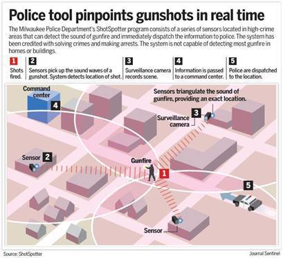
Perhaps the most famous system is ShotSpotter [2], the leader in the United States in detecting shots from a firearm in an urban setting. Directional microphones were installed in the most dangerous areas (on poles, houses, and other tall buildings) that capture the sounds of the city background. In the case of a positive shot identification, information from the GPS coordinates of a specific microphone is transmitted to the central computer, where additional sound analysis is performed to screen out possible false alarms, such as a flying helicopter or, for example, an exploding firecracker. If the shot is confirmed, the patrol leaves on the spot. The system installed in Washington in 2006, over the years, localized 39,000 shots from firearms, and the police were able to quickly respond in each case. [3]
')


Among the service providers of audio analysis in the Russian Federation can be identified "SistemaSarov" [4]. The acoustic monitoring system allows you to automatically allocate acoustic artifacts in the audio stream, perform their preliminary classification (according to the type of alarm event), and in case the terminal device is equipped with a GPS / GLONASS signal receiver, determine the coordinates of the event and save the events to the archive. [five]



The project "AudioAnalytics" [6], based in the UK, provides several solutions for different use cases. The architecture of the proposed solutions is as follows: the CoreLogger program, running on the end-user device, allows receiving and displaying / storing alarm events. It works in conjunction with another part of the overall system - Sound Packs - which is nothing more than a set of various audio analytics modules. The main features of these modules are the detection of the following audio events:

• aggression (talking on high tones, cry);
• car alarm;
• breaking glass;
• search for keywords (“police”, “help”, etc.);
• shots;
• cry / cry baby.

Additionally, a part of the system called Core Trainer is provided, which, based on the set of audio signals submitted to it, will select the most different (prominent) parts and form a new pattern for SoundPacks.

Methods and approaches to detecting and recognizing audio events of various types (shot, broken glass, scream)

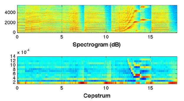
As an example of the initial data, spectrograms of three different types of audio events are presented:
1. A set of shots.


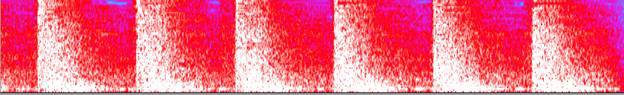
2. Broken glass


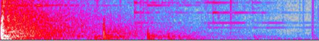
3. Scream


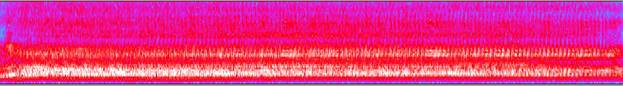
The corresponding audio recordings are downloaded from the audio database [7]. Other sources of source audio data include databases [8] [9] [10] [11].
The task of recognizing various disturbing audio events is divided into 2 subtasks [12]:

• detection (extraction) of sharp impulse signals from background noise in the audio data stream;
• classification (recognition) of the detected signal to one of the types of audio events.

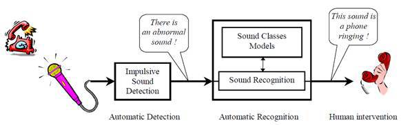
Detection of impulsive eye-catching audio events

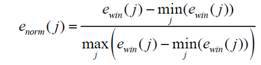
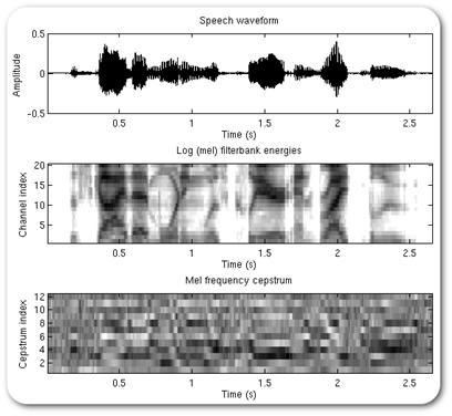
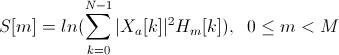
Most methods are based on determining the power for a set of consecutive non-overlapping blocks of audio signal [13]. The power for the k-th block of a signal consisting of for N samples is defined as




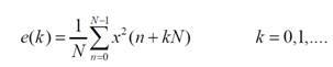
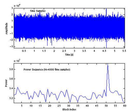
As an example, an audio signal with a shot that occurred at 4.6 s is given, as well as a set of power values ​​for blocks of N = 4000 samples, which corresponds to the duration of each block of about 90 ms.
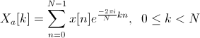
Various methods differ in the method of automatic detection of a block corresponding to a sharp pulse sound:
based on the standard deviation of the normalized power values ​​of the blocks;
based on the application of a median filter for block power values;
over dynamic threshold for block power values.
Let's take a closer look at them:

Method based on standard deviation of normalized block power values

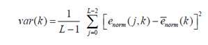
The key aspect of this method is the normalization of the considered set of values ​​of power blocks to the range [0, 1]:



Next, the standard deviation (variance) of the resulting set of values ​​is calculated:




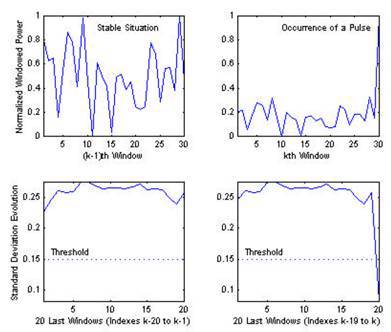
In the case of background noise, the values ​​of the power blocks will be approximately evenly distributed in the range [0-1] (seen in the figure to the left). Since when a new power value is received for an audio signal block, the values ​​are renormalized to the specified range, when a block with a significantly higher power level occurs, the standard deviation value will decrease significantly compared to the same value for a set of previous background power blocks. By reducing the standard deviation below the threshold value, a block with a pulse signal can be automatically detected.

The advantage of this method is its resistance to changes in the noise level, as well as the ability to detect a slowly varying signal by analyzing the average value of the normalized power blocks.

Method based on using median filter

The main stages of automatic detection of pulsed precipitated signals using a median filter are presented below. An example of applying a median filter of order k to the set of power blocks is presented in the figure below.



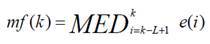
To detect a block with a pulse event, a conditional median filter (conditional median filtering) is applied, which leaves the original signal value if the difference between the original sample and the median value is less than the threshold value, and the median value otherwise.




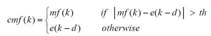
By calculating the difference between the signal after applying the conditional median filter and the shifted source signal, you can automatically select the block with the impulse event that occurred.

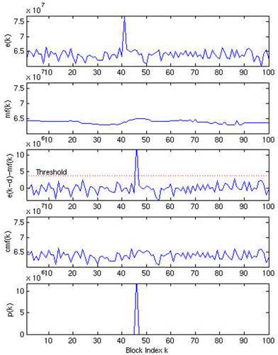
Dynamic threshold method for block power values

In this method, it is proposed to detect a pulsed signal using the average value of the power set of the blocks and the standard deviation as a dynamic threshold. Automatic detection occurs when the power of the next block exceeds the threshold value, defined as

th = par * std + m

Where par is a parameter that determines the sensitivity of the algorithm. An example of using this method with par = 3 is shown in the following figure:

Audio Event Recognition

The general audio event recognition scheme includes the following steps:



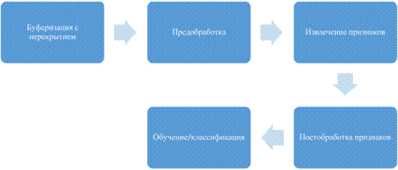
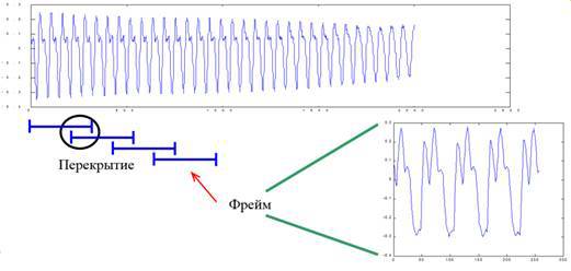
Overlap Buffering

At the first stage, the original audio signal is converted into an overlapping frame set:



Preprocessing stage

The preprocessing stage includes, as a rule, pre-emphasis filtering and window weighting. Pre-emphasis processing is carried out by applying the FIR filter H (z) = 1– a / Z. This is necessary for spectral smoothing of the signal [14]. In this case, the signal becomes less susceptible to various noises arising during processing.

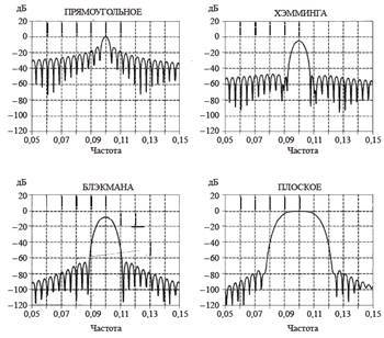
Window weighting should be applied due to the fact that the audio frame is limited in time, therefore, when going into the frequency domain, there will be a side-lobe spectrum filtering effect associated with the shape of the spectrum of the rectangular window function (it looks like sin (x) / x). Therefore, in order to reduce the effect of this effect, weighting of the original signal of different types of windows is applied, with a shape other than rectangular. The samples of the input sequence are multiplied by the corresponding window function, which entails zeroing of the signal values ​​at the edges of the sample. The most commonly used weighted functions are the Hamming, Blackman, Flat, Kaisel-Bessel, Dolph-Chebyshev windows [15]. The spectral characteristics of some are given below:



Feature extraction

There are several approaches to extracting descriptors (features) from an audio signal. All of them are set by the common goal to reduce signal redundancy and highlight the most relevant information, and, at the same time, discard irrelevant information. Typically, features that describe an audio signal from different points of view are combined into one feature vector, on the basis of which the learning process takes place and then classified using the selected trained model. Next will be presented the most popular features extracted from the audio signal.
1. Statistics in the time domain (Time-domain statistics)

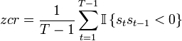
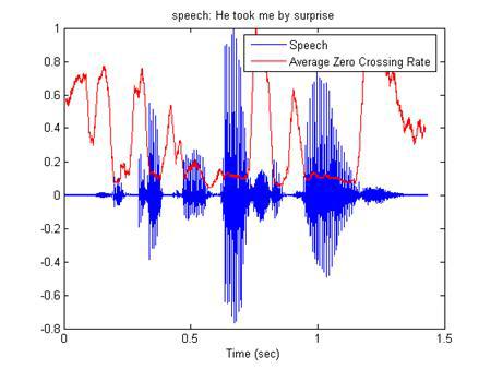
• ZCR (Zero crossing rate) is the number of intersections of the time axis by the audio signal [16].

• Short-time energy [17] - average energy for an audio frame

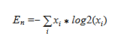
• Entropy of energy [18]

Dividing each frame into a set of sub-frames, the set of energies for each subframe is calculated. Next, normalizing the energy of each of the subframes to the energy of the entire frame, we can consider the set of energies as a set of probabilities and calculate the information entropy using the formula:


2. Frequency domain statistics (Frequency-domain statistic)

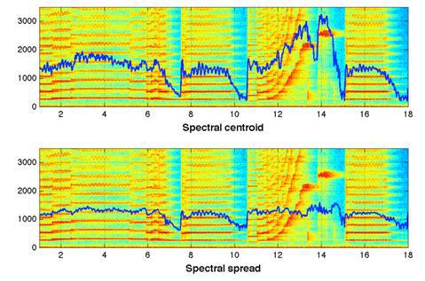
Spectral centroid [17]
It is an interpretation of the "center of mass" of the spectrum. Calculated as the sum of the frequencies weighted by the corresponding amplitudes of the spectrum divided by the sum of the amplitudes:



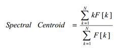
Where F [k] is the amplitude of the spectrum corresponding to the k-th value of the frequency in the DFT spectrum.

Then, the obtained value is conveniently normalized to the maximum frequency (Fs / 2), as a result, the range of possible "center of mass" of the spectrum will lie in the range [0-1].

• Spectrum spread [17] (also called instant spectrum width / bandwidth).

Defined as the second central point:



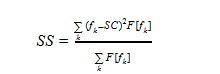
Where fk - values ​​of frequencies in DFT, F [fk] - values ​​of amplitudes, SC - value Spectral centroid

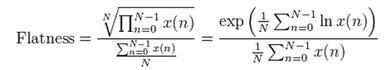
• Audio Spectrum Flatness (ASF) [19]

Reflects the deviation of the power spectrum of the signal from the flat form. From the point of view of human perception, it characterizes the degree of tonality of the sound signal.

• Energy-band spectrum [20]

The frequency space is divided into N bands, after which the spectrum energy is calculated in each band. The values ​​obtained are taken as indications. In essence, the signs in this case represent the value of the energy of the spectrum in the "low resolution".

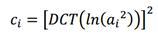
• Cepstral coefficients

Obtained on the basis of the previous signs by transferring them to the cepstral space. A cepstrum is nothing more than the “spectrum spectrum logarithm”; instead of the Fourier transform, use the discrete cosine transform (DCT):

• Spectral entropy

The entropy of the spectrum for a given frame is calculated in a similar way with the entropy of energy in the time domain: the frequency region of the spectrum is divided into N frequency subregions, for each of which the part of the total spectrum energy attributable to this subdomain is calculated, and then the information entropy is calculated by analogy with the time domain.

• Spectral flux [21]

Spectrum Flow - reflects how quickly the energy of the spectrum changes, is calculated based on the spectrum on the current and previous frames. It is defined as the second norm (Euclidean distance) between two normalized spectra:

windowFFT = windowFFT / sum (windowFFT);
F = sum ((windowFFT - windowFFTPrev). ^ 2);

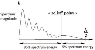
• Spectral rolloff ("collapse" of energy) [22]

It is defined as the relative frequency within which a certain part of the total energy of the spectrum is concentrated (set as parameter c):

countFFT -> c * totalEnergy
SR = countFFT / lengthFFT

A schematic representation of the Spectral rolloff value at c = 0.95:

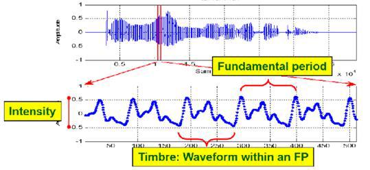
• Signs that reflect the harmony of the audio signal (harmonic ration, fundamental frequency ):

3. MFCC - Mel-frequency cepstral coefficients. (Habra source [23])
The general scheme for obtaining chalk-frequency cepstral coefficients is presented in the following diagram [24].



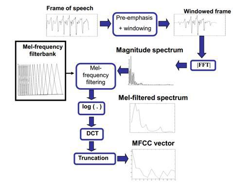
As mentioned earlier, the audio signal is divided into frames, pre-emphasis filtering and window weighting are performed, a fast Fourier transform is performed, then the spectrum is passed through a set of triangular filters evenly spaced on the chalk scale. This leads to a higher density of filters in the low-frequency range and lower density in the high-frequency range, which reflects the sensitivity of the perception of sound signals by the human ear. Thus, the basic information is “removed” from the audio signal in the low-frequency region, which is the most relevant feature of sound signals (especially speech). Next, the samples are transferred to the cepstral space using a discrete cosine transform (DCT).



Mathematical description:

Apply Fourier transform to the signal.



We make a combination of filters using the window function



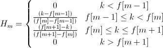
For which the frequency f [m] is obtained from the equality



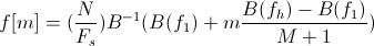
B (b) - conversion of the value of the frequency in the chalk scale, respectively,



We calculate the energy for each window



Apply DCT



4. LPC (Linear prediction coefficients)

The characteristics are coefficients predicting a signal based on a linear combination of previous samples. [25] Essentially, they are coefficients of an FIR filter of the corresponding order:



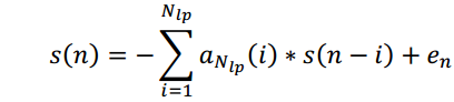
They are also used in speech coding (Linear Prediction Coding), as it has been shown that they well approximate the characteristics of speech signals.

In various articles, the effect of certain components of the feature vector on the recognition quality of audio events is investigated.

Postprocessing signs

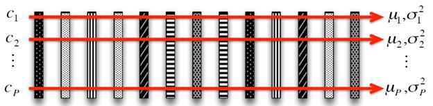
After extracting the necessary features of the signal for their further use, signs are normalized so that each component of the feature vector has an average value of 0 and a standard deviation of 1:



Often used the technique of mid-term analysis [26], when the averaging of signs over a set of successive frames. As a rule, 1-10 seconds is selected as the interval for averaging.



As a rule, the dimension of the feature vector is quite large, which significantly affects the performance of the learning process in the future. That is why in this case, the well-known and theoretically studied methods for reducing the dimension of the feature vector are applied (LDA, PCA, etc.) [27].

One of the advantages of using dimension reduction methods is the ability to significantly increase the speed of the learning process by reducing the number of signs. Moreover, by selecting features that have the best discriminatory abilities in a separate set, it is possible to remove unnecessary, irrelevant information, which will increase the accuracy of machine learning algorithms (such as SVM, etc.) [28]

These methods were addressed in the facial recognition material. The difference between the PCA and LDA methods is that the PCA method allows one to reduce the dimension of the feature vector by identifying independent components that cover the variance in all events as much as possible.



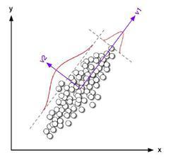
While LDA highlights components that show the best discriminatory abilities among a set of classes.



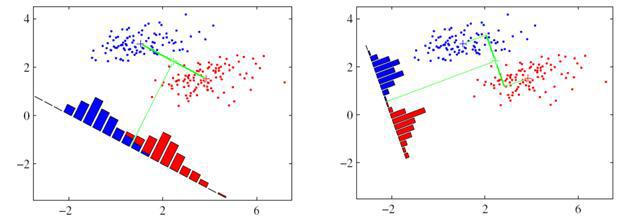
In both the PCA and LDA, at the learning stage, the matrix W is calculated, which determines the linear transformation of the original feature vector to the new space of the reduced dimension Y = WTX

Choosing a classifier

Finally, the last step is the selection of a classifier (training model). Some studies in the field of audio analysis in detecting audio signals of interest are devoted to comparing the recognition accuracy when using different models of classifiers for various types of audio events. It is noted that the use of hierarchical classifiers significantly increases the recognition accuracy in comparison with the use of multi-class classifiers. [29] [19]

The simplest version of the recognition model is the Bayesian classifier , which is based on the calculation of the likelihood function for each of the classes, and at the stage of recognition the event belongs to the class, the posterior probability of which is maximum among all classes. The following figure shows an example of classification for a feature vector of dimension 2. Ellipses are centered with respect to the mean values ​​corresponding to each of the classes, the red borders are a set of feature values ​​where the classes are equivalent.



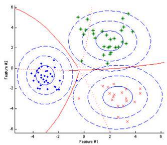
In the case of selecting features that show good discriminatory properties, a high recognition result can be achieved using Bayesian classifiers.

In contrast to the classical Bayesian classifier, where the parameters of the Gaussian distribution were used for the approximation of each class, the “mix” of several Gaussians [19] is used as a function of the probability distribution density in GMM (Gaussian Mixture Model) [19]; learning using the EM (Expectation Maximization) algorithm. As can be seen from the figure representing the result of the classification of the three classes, the area of ​​space corresponding to each class is a more complex shape than the ellipse, the recognition model has become more accurate, respectively, the recognition result will improve.



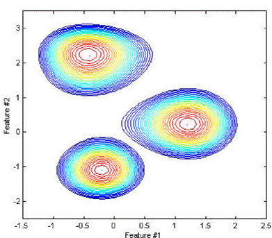
Among the shortcomings of this model, it is possible to note the high sensitivity to variations in the training sample of data when choosing a large number of Gaussian distributions, which can lead to a retraining process.

SVM (Support Vector Machine) classifier [30], which translates the original feature vectors into a space with a higher dimension and finds the maximum separation from recognizable classes, is another way to classify the attributes extracted from an audio signal. Not only a linear function, but also a polynomial function, as well as RBF (radial-basis function) [31], can act as the core.



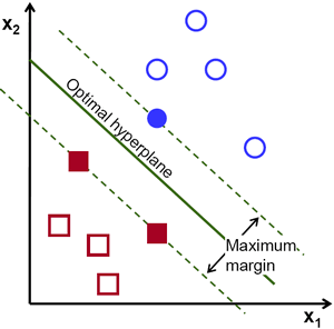
The advantage of this classifier is that at the stage of learning the method finds a band of maximum width, which at the stage of recognition will allow a more accurate classification. Among the shortcomings can be identified sensitivity to data standardization and noise.

The use of HMM (Hidden Markov Model) [32] and neural networks [27] as a classifier was considered in our previous review of face recognition algorithms (Habraistochnik [33]).

A page about audio analytics on the company's website .

Bibliography

[1] "http://www.secuteck.ru/articles2/videonabl/10-trendov-videonablyudeniya-2014po-versii-kompanii-ihs/," [On the Internet].
[2] "http://www.shotspotter.com/," [On the Internet].
[3] "http://habrahabr.ru/post/200850/," [On the Internet].
[4] "http://sarov-itc.ru/," [On the Internet].
[5] "http://sarov-itc.ru/docs/acoustic_monitoring_description.pdf," [On the Internet].
[6] “http://www.audioanalytic.com/,” [On the Internet].
[7] "http://www.freesound.org/," [On the Internet].
[8] “http://sounds.bl.uk/,” [On the Internet].
[9] "http://www.pdsounds.org/," [On the Internet].
[10] “http://macaulaylibrary.org/,” [On the Internet].
[11] "http://www.audiomicro.com/," [On the Internet].
[12] A. Dufaux, "Automatic Sound Detection And Recognition For Noisy Environment.".
[13] IL Freire, “Gunshot detection in noisy environments”.
[14] F. Capman, "Abnormal audio event detection."
[15] Mikulovich, “Digital Signal Processing,” [On the Internet].
[16] L. Gerosa, “SCREAM AND GUNSHOT DETECTION IN NOISY ENVIRONMENTS”.
[17] C. Clavel, “EVENTS DETECTION FOR AN AUDIO-BASED SURVEILLANCE SYSTEM”.
[18] A. Pikrakis, "GUNSHOT DETECTION IN AUDIO STREAMS FROM MOVIES BY MEANS OF DYNAMIC PROGRAMMING AND BAYESIAN NETWORKS".
[19] S. Ntalampiras, "ON ACOUSTIC SURVEILLANCE OF HAZARDOUS SITUATIONS".
[20] MF McKinney, "AUTOMATIC SURVEILLANCE OF THE ACOUSTIC ACTIVITY IN OUR LIVING".
[21] D. Conte, “An ensemble of rejecting classifiers for anomaly detection of audio events”.
[22] G. Valenzise, ​​“Screaming and Gunshot Detection and Localization for Audio Surveillance Systems”.
[23] “http://habrahabr.ru/post/140828/,” [On the Internet].
[24] I. Paraskevas, "Feature Extraction for Audio Classification of Gunshots Using the Hartley Transform".
[25] W. Choi, “Selective Background Adaptation Based Abnormal Acoustic Event Recognition for Audio Surveillance.”
[26] T. Giannakopoulos, "Realtime depression estimation using mid-term audio features," [On the Internet].
[27] J. Port-elo, “NON-SPEECH AUDIO EVENT DETECTION”.
[28] B. Uzkent, "NON-SPEECH ENVIRONMENTAL SOUND CLASSIFICATION USING SVMS WITH A NEW SET OF FEATURES".
[29] PK Atrey, "AUDIO BASED EVENT DETECTION FOR MULTIMEDIA SURVEILLANCE".
[30] A. Kumar, “AUDIO EVENT DETECTION FROM ACOUSTIC UNIT OCCURRENCE PATTERNS”.
[31] T. Ahmed, "IMPROVING EFFICIENCY AND RELIABILITY OF GUNSHOT DETECTION SYSTEMS".
[32] M. Pleva, “Automatic detection of audio events indicating threats”.
[33] "http://habrahabr.ru/company/synesis/blog/238129/," [On the Internet].