Apache Spark Introduction
Hi, Habr!

Last time, we looked at the wonderful Vowpal Wabbit tool, which is useful in cases when you have to study on samples that do not fit in the RAM. Recall that a feature of this tool is that it allows you to build primarily linear models (which, by the way, have a good generalizing ability), and the high quality of the algorithms is achieved through selection and generation of features, regularization and other additional techniques. Today we consider a tool that is more popular and designed for processing large amounts of data - Apache Spark .
We will not go into the details of the history of this instrument, as well as its internal structure. Focus on practical things. In this article we will look at the basic operations and basic things that can be done in Spark, and next time we will take a closer look at the MlLib machine learning library, as well as GraphX for graph processing (the author of this post mainly uses this tool for just the case when it is often necessary to keep a graph in RAM on a cluster, while Vowpal Wabbit is often enough for machine learning). There will not be a lot of code in this manual, since discusses the basic concepts and philosophy of Spark. In the following articles (about MlLib and GraphX) we will take some dataset and take a closer look at Spark in practice.
')
At once, we say that Spark natively supports Scala , Python and Java . Examples will be considered in Python, because it is very convenient to work directly in IPython Notebook , unloading a small part of the data from the cluster and processing, for example, with the Pandas package - you get a rather convenient bundle
Let's start with the fact that the basic concept in Spark is RDD (Resilient Distributed Dataset) , which is a Dataset, on which you can do two types of transformations (and, accordingly, all the work with these structures is in the sequence of these two actions) .
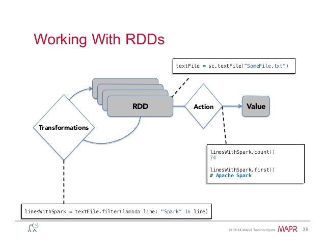
The result of applying this operation to RDD is a new RDD. As a rule, these are operations that in some way convert the elements of a given dataset. Here is the incomplete of the most common transformations, each of which returns a new dataset (RDD):
.map (function) - applies function function to each element of dataset
.filter (function) - returns all elements of the dataset on which the function function returns the true value
.distinct ([numTasks]) - returns a dataset that contains unique elements of the source dataset
It is also worth noting about operations on sets, the meaning of which is clear from the names:
.union (otherDataset)
.intersection (otherDataset)
.cartesian (otherDataset) - the new dataset contains all sorts of pairs (A, B), where the first element belongs to the original dataset, and the second one - to the dataset argument
Actions are applied when it is necessary to materialize the result - as a rule, save the data to disk, or output part of the data to the console. Here is a list of the most common actions that can be applied over RDD:
.saveAsTextFile (path) - saves data to a text file (in hdfs, to a local machine or to any other supported file system - a full list can be found in the documentation)
.collect () - returns dataset elements as an array. As a rule, this is used in cases when there is little data in the dataset (various filters and transformations are applied) - and visualization or additional data analysis is necessary, for example, using the Pandas package
.take (n) - returns the first n dataset elements as an array
.count () - returns the number of elements in dataset
.reduce (function) is a familiar operation for those familiar with MapReduce . From the mechanism of this operation, it follows that the function function (which takes 2 arguments as an input returns one value) must be commutative and associative
These are the basics you need to know when working with a tool. Now let's do a little practice and show you how to load data into Spark and do simple calculations with it.
When you start Spark, the first thing you need to do is create a SparkContext (in simple terms, an object that is responsible for implementing lower-level operations with a cluster — see the documentation for details), which is automatically created when you start Spark-Shell. ( sc object)
You can upload data to Spark in two ways:
but). Directly from a local program using the .parallelize (data) function
b). From supported storages (for example, hdfs) using the .textFile (path) function
At this point, it is important to note one feature of data storage in Spark and at the same time the most useful function .cache () (partly due to which Spark became so popular), which allows you to cache data in RAM (taking into account the availability of the latter). This allows you to perform iterative calculations in memory, thereby getting rid of IO-overhead. This is especially important in the context of machine learning and graphing; most algorithms are iterative, ranging from gradient methods to algorithms such as PageRank
After loading the data in RDD, we can do various transformations and actions on it, as mentioned above. For example:
Let's look at the first few elements:
Either we immediately load these elements into Pandas and work with the DataFrame:
In general, as you can see, Spark is so convenient that further, probably there is no point in writing various examples, or you can just leave this exercise to the reader - many calculations are written literally in a few lines.
Finally, we will show only an example of transformation, namely, we calculate the maximum and minimum elements of our dataset. As you can easily guess, this can be done, for example, using the .reduce () function:
So, we have reviewed the basic concepts needed to work with the tool. We did not consider working with SQL, working with pairs <key, value> (what is done is easy - to do this, first apply a filter to RDD, for example, to select the key, and then it’s easy to use built-in functions like sortByKey , countByKey , join , etc.) - the reader is invited to familiarize himself with this, and if you have questions, write in a comment. As already noted, the next time we will look in detail at the MlLib library and separately - GraphX
Last time, we looked at the wonderful Vowpal Wabbit tool, which is useful in cases when you have to study on samples that do not fit in the RAM. Recall that a feature of this tool is that it allows you to build primarily linear models (which, by the way, have a good generalizing ability), and the high quality of the algorithms is achieved through selection and generation of features, regularization and other additional techniques. Today we consider a tool that is more popular and designed for processing large amounts of data - Apache Spark .
We will not go into the details of the history of this instrument, as well as its internal structure. Focus on practical things. In this article we will look at the basic operations and basic things that can be done in Spark, and next time we will take a closer look at the MlLib machine learning library, as well as GraphX for graph processing (the author of this post mainly uses this tool for just the case when it is often necessary to keep a graph in RAM on a cluster, while Vowpal Wabbit is often enough for machine learning). There will not be a lot of code in this manual, since discusses the basic concepts and philosophy of Spark. In the following articles (about MlLib and GraphX) we will take some dataset and take a closer look at Spark in practice.
')
At once, we say that Spark natively supports Scala , Python and Java . Examples will be considered in Python, because it is very convenient to work directly in IPython Notebook , unloading a small part of the data from the cluster and processing, for example, with the Pandas package - you get a rather convenient bundle
Let's start with the fact that the basic concept in Spark is RDD (Resilient Distributed Dataset) , which is a Dataset, on which you can do two types of transformations (and, accordingly, all the work with these structures is in the sequence of these two actions) .
Transformations
The result of applying this operation to RDD is a new RDD. As a rule, these are operations that in some way convert the elements of a given dataset. Here is the incomplete of the most common transformations, each of which returns a new dataset (RDD):
.map (function) - applies function function to each element of dataset
.filter (function) - returns all elements of the dataset on which the function function returns the true value
.distinct ([numTasks]) - returns a dataset that contains unique elements of the source dataset
It is also worth noting about operations on sets, the meaning of which is clear from the names:
.union (otherDataset)
.intersection (otherDataset)
.cartesian (otherDataset) - the new dataset contains all sorts of pairs (A, B), where the first element belongs to the original dataset, and the second one - to the dataset argument
Actions
Actions are applied when it is necessary to materialize the result - as a rule, save the data to disk, or output part of the data to the console. Here is a list of the most common actions that can be applied over RDD:
.saveAsTextFile (path) - saves data to a text file (in hdfs, to a local machine or to any other supported file system - a full list can be found in the documentation)
.collect () - returns dataset elements as an array. As a rule, this is used in cases when there is little data in the dataset (various filters and transformations are applied) - and visualization or additional data analysis is necessary, for example, using the Pandas package
.take (n) - returns the first n dataset elements as an array
.count () - returns the number of elements in dataset
.reduce (function) is a familiar operation for those familiar with MapReduce . From the mechanism of this operation, it follows that the function function (which takes 2 arguments as an input returns one value) must be commutative and associative
These are the basics you need to know when working with a tool. Now let's do a little practice and show you how to load data into Spark and do simple calculations with it.
When you start Spark, the first thing you need to do is create a SparkContext (in simple terms, an object that is responsible for implementing lower-level operations with a cluster — see the documentation for details), which is automatically created when you start Spark-Shell. ( sc object)
Data loading
You can upload data to Spark in two ways:
but). Directly from a local program using the .parallelize (data) function
localData = [5,7,1,12,10,25] ourFirstRDD = sc.parallelize(localData) b). From supported storages (for example, hdfs) using the .textFile (path) function
ourSecondRDD = sc.textFile("path to some data on the cluster") At this point, it is important to note one feature of data storage in Spark and at the same time the most useful function .cache () (partly due to which Spark became so popular), which allows you to cache data in RAM (taking into account the availability of the latter). This allows you to perform iterative calculations in memory, thereby getting rid of IO-overhead. This is especially important in the context of machine learning and graphing; most algorithms are iterative, ranging from gradient methods to algorithms such as PageRank
Work with data
After loading the data in RDD, we can do various transformations and actions on it, as mentioned above. For example:
Let's look at the first few elements:
for item in ourRDD.top(10): print item Either we immediately load these elements into Pandas and work with the DataFrame:
import pandas as pd pd.DataFrame(ourRDD.map(lambda x: x.split(";")[:]).top(10)) In general, as you can see, Spark is so convenient that further, probably there is no point in writing various examples, or you can just leave this exercise to the reader - many calculations are written literally in a few lines.
Finally, we will show only an example of transformation, namely, we calculate the maximum and minimum elements of our dataset. As you can easily guess, this can be done, for example, using the .reduce () function:
localData = [5,7,1,12,10,25] ourRDD = sc.parallelize(localData) print ourRDD.reduce(max) print ourRDD.reduce(min) So, we have reviewed the basic concepts needed to work with the tool. We did not consider working with SQL, working with pairs <key, value> (what is done is easy - to do this, first apply a filter to RDD, for example, to select the key, and then it’s easy to use built-in functions like sortByKey , countByKey , join , etc.) - the reader is invited to familiarize himself with this, and if you have questions, write in a comment. As already noted, the next time we will look in detail at the MlLib library and separately - GraphX
Source: https://habr.com/ru/post/250811/
All Articles