Machine learning - 1. Correlation and regression. Example: site visitors conversion
As promised, I begin the cycle of articles on "machine learning". This will be devoted to such concepts from statistics as the correlation of random variables and linear regression. Consider both real data and model data (Monte-Carlo simulation).
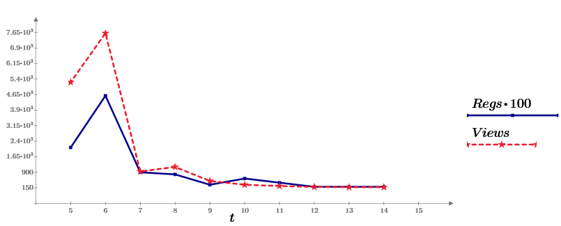
To make it more interesting, the story is built on examples, and as data (and in this, and in the following, articles) I will try to take statistics straight from here, with Habr. Namely, a week ago I wrote my first article on Habré (about Mathcad Express, in which we will count everything). And now the statistics on its views for 10 days and offer as source data. On the graph, this is the Views series, the blue line. The second data series (Regs, with a factor of 100) shows the number of readers who have performed a certain action after reading (registration and download of the Mathcad Prime distribution).
')
It just so happened that I, besides the statistics of viewing the article (from Habr), had access to the statistics of downloads of Mathcad (by the link I gave inside the text of the article). Thus, we have everything in order to deal with such a concept of Internet marketing, as a conversion . Conversion is usually called the ratio of the number of site visitors who completed a purchase, registration, or the like. to the total number of visitors. For example: on the first day of publication my article was viewed 5 thousand times, and there were 20 downloads, i.e. conversion was 0.4%.
All pictures are screenshots of Mathcad Express (you can take the calculations here , repeat them, and if you want to change them and use them for your needs). I entered the initial data (three vectors) with my hands:
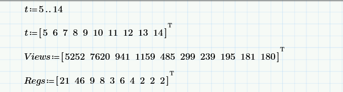
Here are the calculations for conversion (in%): “instantaneous” (for each day) and “average” (for 10 days). It is curious that the conversion value “floats” a bit over time (from 0.4% on the first day to a quasi-stationary 1% in the last days), which, by itself, is worthy of discussion (which we will postpone until the following articles about random processes and correlation time ).
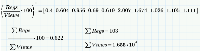
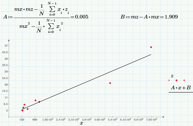
The obvious fact that the number of targeted actions (downloads) depends on the number of views, clearly shows the chart Regs (Views). We see that, although both the number of views and the number of downloads are random, they are nevertheless linked by (almost) linear dependence.
Now a bit of “school” statistics: the calculation (by definition) of the mean, variance and correlation coefficient of two Views and Regs samples.
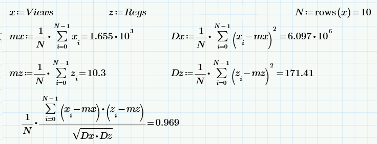
The last formula is the calculation of the correlation coefficient — measures of how dependent two random variables are (more precisely, measures of linear dependence). It turns out that the sample value of the correlation coefficient is 0.97. This is a lot (which, however, is not surprising, by the very formulation of the problem).
Finally, we solve a mathematical regression problem — an approximation, in the general case, of data sampling (x, z) by a certain function f (x), which minimizes in a certain way the set of errors f (x) -z. The simplest and most frequently used type of regression is linear, when f (x) = A * x + B. Another linear regression is often called the least squares method, since the coefficients A and B are usually calculated from the condition of minimizing the sum of squares of errors:
By the way, the method of least squares (minimizing the sum of squares of errors) is not the only possible option to construct a regression. For example, median-median linear regression is sometimes used.
Finally, about why we need regression in our problem. If we take the linear nature of the dependence of downloads on views, then the coefficient A will just characterize the conversion. Judging by it, the conversion is 0.005 = 0.5%, that is, if, for example, we have a marketing goal - to reach 100 downloads, then, based on the linear regression model, we need to “upload” to the site 100 / 0.005 = 20 thousand views.
While in the last part we operated on random data obtained during the experiment, in conclusion we will repeat the same calculations using the pseudo-random number sensor. In Monte Carlo methods, it is often required to create random numbers with a specific correlation. To begin with, we will generate three pseudo-random arrays: x and y are independent, and z is dependent on x (with the “general” value of the correlation coefficient r):
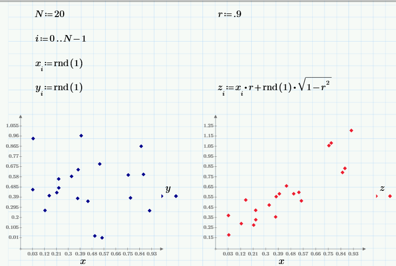
The graph on the left shows the dependence of uncorrelated random values of x and y, and on the right the dependence of correlated z and x.
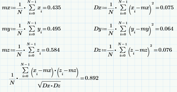
Using the same formulas as in the last section, we obtain the statistical characteristics of the samples x, y, and z (including the sample value of the correlation coefficient):
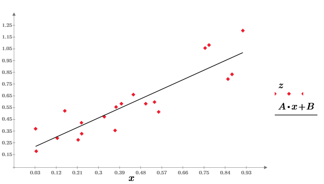
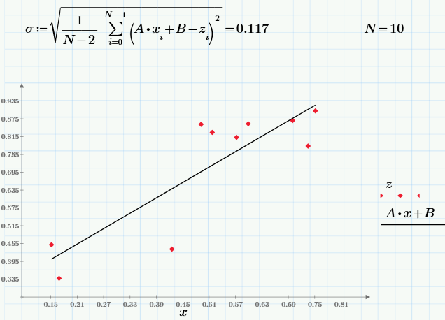
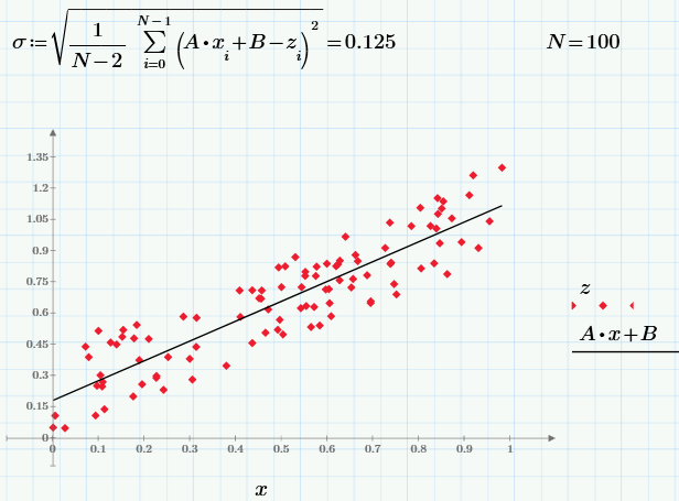
Well, and finally, using the least squares formula, we construct a linear regression z = A * x + B:
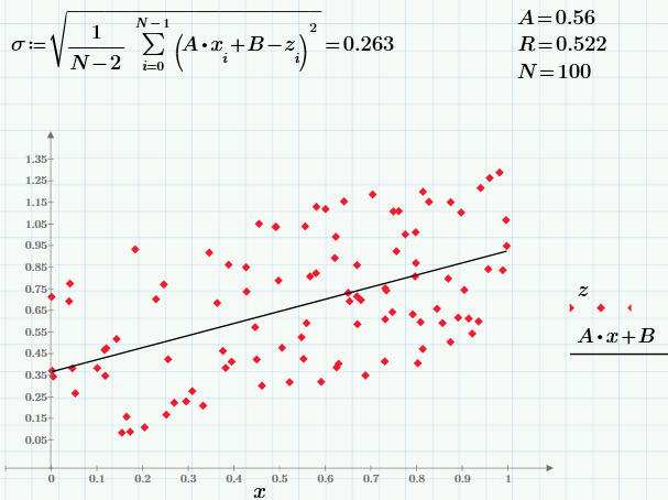
Interested readers leave experimenting with the parameter r and see how its change will affect the dependence z (x). It is still curious, changing the sample size N, to follow the result of the calculation of statistical characteristics.
References:
Part 1. Real data
To make it more interesting, the story is built on examples, and as data (and in this, and in the following, articles) I will try to take statistics straight from here, with Habr. Namely, a week ago I wrote my first article on Habré (about Mathcad Express, in which we will count everything). And now the statistics on its views for 10 days and offer as source data. On the graph, this is the Views series, the blue line. The second data series (Regs, with a factor of 100) shows the number of readers who have performed a certain action after reading (registration and download of the Mathcad Prime distribution).
')
It just so happened that I, besides the statistics of viewing the article (from Habr), had access to the statistics of downloads of Mathcad (by the link I gave inside the text of the article). Thus, we have everything in order to deal with such a concept of Internet marketing, as a conversion . Conversion is usually called the ratio of the number of site visitors who completed a purchase, registration, or the like. to the total number of visitors. For example: on the first day of publication my article was viewed 5 thousand times, and there were 20 downloads, i.e. conversion was 0.4%.
All pictures are screenshots of Mathcad Express (you can take the calculations here , repeat them, and if you want to change them and use them for your needs). I entered the initial data (three vectors) with my hands:
Here are the calculations for conversion (in%): “instantaneous” (for each day) and “average” (for 10 days). It is curious that the conversion value “floats” a bit over time (from 0.4% on the first day to a quasi-stationary 1% in the last days), which, by itself, is worthy of discussion (which we will postpone until the following articles about random processes and correlation time ).
The obvious fact that the number of targeted actions (downloads) depends on the number of views, clearly shows the chart Regs (Views). We see that, although both the number of views and the number of downloads are random, they are nevertheless linked by (almost) linear dependence.
Now a bit of “school” statistics: the calculation (by definition) of the mean, variance and correlation coefficient of two Views and Regs samples.
The last formula is the calculation of the correlation coefficient — measures of how dependent two random variables are (more precisely, measures of linear dependence). It turns out that the sample value of the correlation coefficient is 0.97. This is a lot (which, however, is not surprising, by the very formulation of the problem).
Finally, we solve a mathematical regression problem — an approximation, in the general case, of data sampling (x, z) by a certain function f (x), which minimizes in a certain way the set of errors f (x) -z. The simplest and most frequently used type of regression is linear, when f (x) = A * x + B. Another linear regression is often called the least squares method, since the coefficients A and B are usually calculated from the condition of minimizing the sum of squares of errors:
By the way, the method of least squares (minimizing the sum of squares of errors) is not the only possible option to construct a regression. For example, median-median linear regression is sometimes used.
Finally, about why we need regression in our problem. If we take the linear nature of the dependence of downloads on views, then the coefficient A will just characterize the conversion. Judging by it, the conversion is 0.005 = 0.5%, that is, if, for example, we have a marketing goal - to reach 100 downloads, then, based on the linear regression model, we need to “upload” to the site 100 / 0.005 = 20 thousand views.
Part 2. Monte-Carlo simulation
While in the last part we operated on random data obtained during the experiment, in conclusion we will repeat the same calculations using the pseudo-random number sensor. In Monte Carlo methods, it is often required to create random numbers with a specific correlation. To begin with, we will generate three pseudo-random arrays: x and y are independent, and z is dependent on x (with the “general” value of the correlation coefficient r):
The graph on the left shows the dependence of uncorrelated random values of x and y, and on the right the dependence of correlated z and x.
Using the same formulas as in the last section, we obtain the statistical characteristics of the samples x, y, and z (including the sample value of the correlation coefficient):
Well, and finally, using the least squares formula, we construct a linear regression z = A * x + B:
Interested readers leave experimenting with the parameter r and see how its change will affect the dependence z (x). It is still curious, changing the sample size N, to follow the result of the calculation of statistical characteristics.
References:
- Video Course "Machine Learning" (ShAD Yandex)
- Gareth James, Daniela Witten, Trevor Hastie, Robert Tibshirani. An Introduction to Statistical Learning in R (PDF)
- Trevor Hastie, Robert Tibshirani, Jerome Friedman. The Elements of Statistical Learning (PDF)
Source: https://habr.com/ru/post/250633/
All Articles