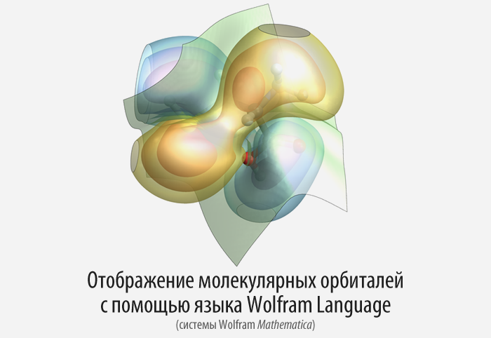
Displaying molecular orbitals using the Wolfram Language (Mathematica)

Translation of Jason B.'s post " Plotting electronic orbitals using Mathematica ".

I express my gratitude for the help in translating Wolfram Mathematica to the member of the VKontakte community of Russian-language support Kurban Magomedov .

Download the translation in the form of a Mathematica document, which contains all the code used in the article, as well as additional materials, here .



Chemists are often useful image of molecular orbitals (MO). They are used to describe the wave function of electrons in atoms or molecules. As a rule, these are the results of various quantum-chemical or quantum-physical calculations performed in specialized software for the calculation of MOs, which are presented in the form of a cube-file developed by Gaussian . These files contain volumetric data for building orbitals on a three-dimensional grid.



There are many applications for viewing cube-files, such as VMD or GaussView , but I would like to use Mathematica's features, which it provides for combining and creating various types of graphic objects, as well as automating the entire process, which ultimately allowed creating effective frames for video in which you can observe a change in MO.

')





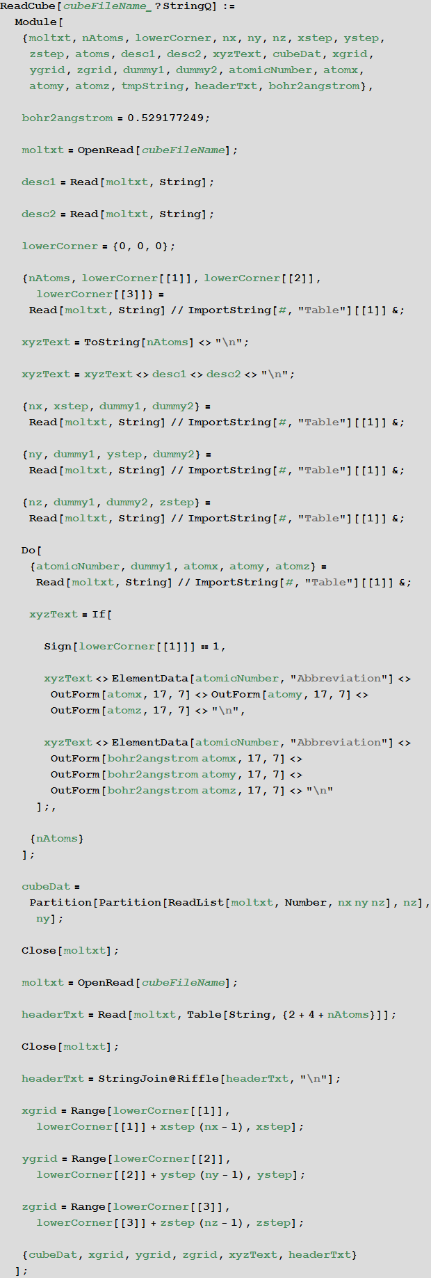
First of all, we need a function to extract data from a cube file. In the process, we will also create text for the XYZ file (format, also presented by Gaussian). The OutForm function essentially simulates the operation of PRINTF functions found in other programming languages.



In [1]: =







Import cude file:



In [2]: =







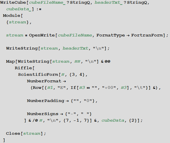
If you need to create a cube-file, you can use the following function:



In [3]: =







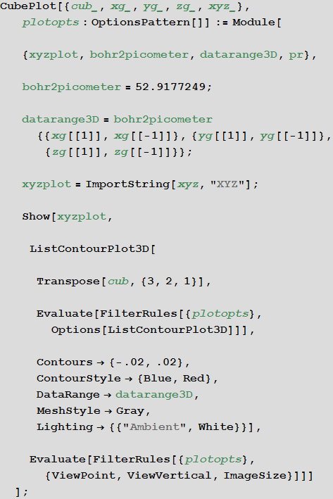
Next we need the MO display function:



In [4]: ​​=







Let's now look at how things work with an example. Take some cude-file, say, cys-MO35.cube and import data from it:



In [5]: =







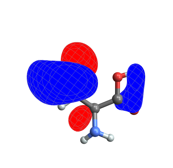
Now we will build a three-dimensional model:



In [6]: =







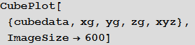
Out [6] =







If you need to create a video file, you will need a set of images with the same viewpoint, which can be set using the ViewAngle , ViewPoint , and ViewCenter options . When you specify these options with their values ​​inside the CubePlot function, it passes them directly to the Show function, which allows you to use the standard Wolfram Language functions in your display function MO:



In [7]: =







Out [8] =







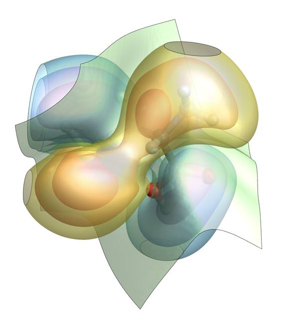
Finally, you can also use any options that the ListContourPlot3D built-in function has :



In [9]: =







Out [9] =







In [10]: =







Out [10] =







Resources for learning Wolfram Language (Mathematica) in Russian: habrahabr.ru/post/244451