Normal-oriented Hemisphere SSAO for Dummies
Hi, username! After a short break, you can again take up three-dimensional graphics. This time we will talk about such a global shading algorithm as the Normal-oriented Hemisphere SSAO . Interesting? Under the cat!
I refused to use XNA, I began to miss the power of the DX9: of course, in general, nothing has changed, but writing the code has become much less crutch. All the following examples will be implemented using the SharpDX.Toolkit framework: do not worry, this is the spiritual heir to XNA , also OpenSource and with support for DX11 .
')
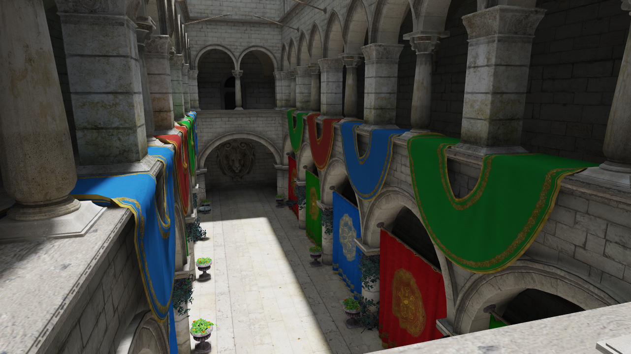
The most important part in the graphics engine of any game (which has claims to be realistic) is lighting. Now it is impossible to completely simulate the lighting in a real-time game as it happens in our real world. Relatively speaking, not in real-time applications: the lighting is considered to be “launching” photons from a light source in the right directions and registering these photons with a camera (eye). For real-time processes like this, apromixing is required, for example: we have a certain surface and a light source, and in order to create lighting, we need to calculate the “illumination” of each pixel of the surface, i.e. only the direct influence of the light source on the texel is taken into account. This apromix does not take into account indirect lighting, i.e. in the case of real-time, a photon can be reflected from a surface and affect another Texel. For single, small light sources this is not particularly critical, but it is worth taking a large light source and an “infinitely distant”, for example, the sun (the sky acts as a powerful “lens” of light from the sun), then problems arise immediately, something like this:
In the real world, on a similar scene, there would not be such blackness in places of shadows. Further developing the theme, you can enter a certain ambient value, which will display the overall illumination of the entire scene, a kind of approximation of indirect illumination. But the fact is that similar lighting throughout the stage is the same everywhere, even in those places where indirect light will have the least impact. But even here you can cheat and complicate apromixing by shading those areas where the reflected light is the most difficult to reach. Thus, we come to a concept called “global shading” ( ambient occlusion ). The essence of this approach is that for each fragments of the scene we find some blocking factor, i.e. the number of non-barred directions of the fall of the "photon" divided by the total number of various directions.
Consider the following picture:

Here we have two points in question, which form a circle with a radius R around it. And in order to determine the degree of obstruction of the taken fragment, it suffices to find the area of the unlocked space and divide by the total area of the circle. If we perform a similar operation for all points of the scene, we will get global shading. It will look something like this (for the three-dimensional case):

But now you need to think about how to implement a similar algorithm in the pipe-line render of the graphics pipeline. The difficulty arises in the fact that geometry drawing occurs gradually. As a result, the first object in the scene will not know about the existence of others. You can, of course, calculate the AO in advance (at the stage of loading) for the scene, but in this case we will not take into account the dynamically changing geometry: physical objects, characters, etc. And here comes the work with the geometry in the screen space (Screen Space). I already mentioned it when talking about the SSLR-algorithm. This can be used and read AO in screen space. Here comes the most classic implementation of SSAO, it was invented by cool guys from kortek exactly 8 years ago. Their algorithm was as follows: after drawing all the geometry, they had a depth buffer, which carries information about all the visible geometry, building spheres for each texel, they counted the number of shading for the scene:

Here, by the way, there is another difficulty. The fact is that we cannot take absolutely all directions into account in real-time, firstly, because space is discrete, and secondly, a cross can be put on performance. We can not even take into account 250 directions (namely, so much is necessary for the minimum imputed image quality). In order to reduce the number of samples - use some core directions (from 8 to 32), which rotate each time at a random value. After these operations, AO is available to us in real time:

The hardest thing in the SSAO algorithm is the definition of a barrier, because it is a reading from a float texture.
A bit later, a modification of the SSAO: Normal-oriented Hemisphere SSAO algorithm was invented. The essence of the modification is that we can increase the accuracy of the algorithm by taking into account the normals (in fact, we need a GBuffer ). For the sample space, we will use not a sphere, but a hemisphere that is oriented along the normal of the current texel. This approach allows you to increase the number of useful samples in two.

If you look at the picture, you can understand what I'm saying:

The final stage of the algorithm will be the blurring of the AO image in order to remove the noise caused by random samples. Ultimately, the implementation of our algorithm will look like this:

With theory so far everything is clear, you can go to practice.
I advise you to read this article, there I talked about the essence of the work of Screen Space space. But, in practice, I will cite very important parts of the code with the necessary comments.
The first thing we need is geometry information: GBuffer . Since its construction is not included in the topic of the article - I will talk about it in detail some other time.
The second is a hemisphere with random directions:
It is important to note that in the shader we will not have a trace, since we are very limited in instructions, instead of this - we will consider the fact of finding the end point in any geometry, therefore it is necessary to take into account more near geometry than far. To do this, it suffices to take a set of points with a normal distribution in the hemisphere. This can be obtained by fair normal distribution, you can simply multiply the vector by a random number from 0 to 1, and you can use a small hack: set the length of a function, for example, a quadratic one. This will give us a better “grade” of the core.
The third is a set of some random vectors, in order to vary the final samples, in my case it is generated in a random way:
But it looks like this:
You should not use such a texture more than 4x4-8x8, because such a rotation of the core gives a low-frequency noise, which is much easier to blur in the future.
Now let's look at the SSAO shader body:
Here we get a non-linear depth, we get the world position and the normal, we get a set of random vectors stretched across the screen. It should immediately say in advance about the two hacks.
The first is that we shift the texel position by the normal multiplied by some small value, this is necessary in order to get rid of unnecessary intersections due to the discreteness of the screen space of the space:
And the second is that in the algorithm we need to compare the depth values, and the nonlinear depth at medium-long distances is in the vicinity of the unit. In an amicable way, we should linearize this depth, but since such values are used only for comparison - you can enter a certain estimate of non-linear depth:
We should also say that it would be good to make a unroll cycle, since The number of samples is known in advance; such code will work faster.
Then the algorithm itself begins:
Rotate the core and orient this core along the normal in the textile:
And we pass the functions of the calculation of the barrier:
We take a sample and design it into the screen space (we obtain new UV.xy values and non-linear depth):
The projection function is as follows:
Constants 0.5f ask for them to be stitched into a matrix.
After that we get a new depth value:
We define the barrage fact as “whether the point is visible to the observer”, i.e. if the point does not lie in any geometry - then assessReaded will always be strictly less assessProjected .
Well, given the fact that in the screen space is full of such a phenomenon as information lost, we must adjust the amount of shading depending on the distance “penetration” into the geometry. This is necessary so that we do not know anything about geometry beyond the visible part of the screen space:
Well, the final stage, this blur. I will only say that it is impossible to blur the SSAO buffer without taking into account the depth heterogeneity as many do. Also, it would be good to take into account the normal when blurring, like this:
The depthFactor and normalFactor coefficients are taken into account in the blur coefficients.
For a more detailed study - I will leave the full source code here , and for those who like to see with their own eyes the demo here .
By the way, in the demo I intend to leave NORMAL_BIAS equal to zero to see the problem, besides, only geometry is drawn in the GBuffer and there is no normal mapping, which is why z-fighting happens at long distances.
In future articles I will try to highlight other real-time ao algorithms, such as HBAO, HDAO, HBAO + , if this topic is interesting, of course.
Have a good job!
But first a little bit of news.
I refused to use XNA, I began to miss the power of the DX9: of course, in general, nothing has changed, but writing the code has become much less crutch. All the following examples will be implemented using the SharpDX.Toolkit framework: do not worry, this is the spiritual heir to XNA , also OpenSource and with support for DX11 .
')
Classically - theories
The most important part in the graphics engine of any game (which has claims to be realistic) is lighting. Now it is impossible to completely simulate the lighting in a real-time game as it happens in our real world. Relatively speaking, not in real-time applications: the lighting is considered to be “launching” photons from a light source in the right directions and registering these photons with a camera (eye). For real-time processes like this, apromixing is required, for example: we have a certain surface and a light source, and in order to create lighting, we need to calculate the “illumination” of each pixel of the surface, i.e. only the direct influence of the light source on the texel is taken into account. This apromix does not take into account indirect lighting, i.e. in the case of real-time, a photon can be reflected from a surface and affect another Texel. For single, small light sources this is not particularly critical, but it is worth taking a large light source and an “infinitely distant”, for example, the sun (the sky acts as a powerful “lens” of light from the sun), then problems arise immediately, something like this:
In the real world, on a similar scene, there would not be such blackness in places of shadows. Further developing the theme, you can enter a certain ambient value, which will display the overall illumination of the entire scene, a kind of approximation of indirect illumination. But the fact is that similar lighting throughout the stage is the same everywhere, even in those places where indirect light will have the least impact. But even here you can cheat and complicate apromixing by shading those areas where the reflected light is the most difficult to reach. Thus, we come to a concept called “global shading” ( ambient occlusion ). The essence of this approach is that for each fragments of the scene we find some blocking factor, i.e. the number of non-barred directions of the fall of the "photon" divided by the total number of various directions.
Consider the following picture:
Here we have two points in question, which form a circle with a radius R around it. And in order to determine the degree of obstruction of the taken fragment, it suffices to find the area of the unlocked space and divide by the total area of the circle. If we perform a similar operation for all points of the scene, we will get global shading. It will look something like this (for the three-dimensional case):
But now you need to think about how to implement a similar algorithm in the pipe-line render of the graphics pipeline. The difficulty arises in the fact that geometry drawing occurs gradually. As a result, the first object in the scene will not know about the existence of others. You can, of course, calculate the AO in advance (at the stage of loading) for the scene, but in this case we will not take into account the dynamically changing geometry: physical objects, characters, etc. And here comes the work with the geometry in the screen space (Screen Space). I already mentioned it when talking about the SSLR-algorithm. This can be used and read AO in screen space. Here comes the most classic implementation of SSAO, it was invented by cool guys from kortek exactly 8 years ago. Their algorithm was as follows: after drawing all the geometry, they had a depth buffer, which carries information about all the visible geometry, building spheres for each texel, they counted the number of shading for the scene:
Here, by the way, there is another difficulty. The fact is that we cannot take absolutely all directions into account in real-time, firstly, because space is discrete, and secondly, a cross can be put on performance. We can not even take into account 250 directions (namely, so much is necessary for the minimum imputed image quality). In order to reduce the number of samples - use some core directions (from 8 to 32), which rotate each time at a random value. After these operations, AO is available to us in real time:
The hardest thing in the SSAO algorithm is the definition of a barrier, because it is a reading from a float texture.
A bit later, a modification of the SSAO: Normal-oriented Hemisphere SSAO algorithm was invented. The essence of the modification is that we can increase the accuracy of the algorithm by taking into account the normals (in fact, we need a GBuffer ). For the sample space, we will use not a sphere, but a hemisphere that is oriented along the normal of the current texel. This approach allows you to increase the number of useful samples in two.
If you look at the picture, you can understand what I'm saying:
The final stage of the algorithm will be the blurring of the AO image in order to remove the noise caused by random samples. Ultimately, the implementation of our algorithm will look like this:
With theory so far everything is clear, you can go to practice.
Theory free zone
I advise you to read this article, there I talked about the essence of the work of Screen Space space. But, in practice, I will cite very important parts of the code with the necessary comments.
The first thing we need is geometry information: GBuffer . Since its construction is not included in the topic of the article - I will talk about it in detail some other time.
The second is a hemisphere with random directions:
_samplesKernel = new Vector3[128]; for (int i = 0; i < _samplesKernel.Length; i++) { _samplesKernel[i].X = random.NextFloat(-1f, 1f); _samplesKernel[i].Z = random.NextFloat(-1f, 1f); _samplesKernel[i].Y = random.NextFloat(0f, 1f); _samplesKernel[i].Normalize(); float scale = (float)i / (float)_samplesKernel.Length; scale = MathUtil.Lerp(0.1f, 1.0f, scale * scale); _samplesKernel[i] *= scale; } It is important to note that in the shader we will not have a trace, since we are very limited in instructions, instead of this - we will consider the fact of finding the end point in any geometry, therefore it is necessary to take into account more near geometry than far. To do this, it suffices to take a set of points with a normal distribution in the hemisphere. This can be obtained by fair normal distribution, you can simply multiply the vector by a random number from 0 to 1, and you can use a small hack: set the length of a function, for example, a quadratic one. This will give us a better “grade” of the core.
The third is a set of some random vectors, in order to vary the final samples, in my case it is generated in a random way:
Color[] randomNormal = new Color[_randomNormalTexture.Width * _randomNormalTexture.Height]; for (int i = 0; i < randomNormal.Length; i++) { Vector3 tsRandomNormal = new Vector3(random.NextFloat(0f, 1f), 1f, random.NextFloat(0f, 1f)); tsRandomNormal.Normalize(); randomNormal[i] = new Color(tsRandomNormal, 1f); } But it looks like this:
You should not use such a texture more than 4x4-8x8, because such a rotation of the core gives a low-frequency noise, which is much easier to blur in the future.
Now let's look at the SSAO shader body:
float depth = GetDepth(UV); float3 texelNormal = GetNormal(UV); float3 texelPosition = GetPosition2(UV, depth) + texelNormal * NORMAL_BIAS; float3 random = normalize(RandomTexture.Sample(NoiseSampler, UV * RNTextureSize).xyz); float ssao = 0; [unroll] for(int i = 0; i < MAX_SAMPLE_COUNT; i++) { float3 hemisphereRandomNormal = reflect(SamplesKernel[i], random); float3 hemisphereNormalOrientated = hemisphereRandomNormal * sign( dot(hemisphereRandomNormal, texelNormal)); ssao += calculateOcclusion(texelPosition, texelNormal, hemisphereNormalOrientated, RADIUS); } return (ssao / MAX_SAMPLE_COUNT); Here we get a non-linear depth, we get the world position and the normal, we get a set of random vectors stretched across the screen. It should immediately say in advance about the two hacks.
The first is that we shift the texel position by the normal multiplied by some small value, this is necessary in order to get rid of unnecessary intersections due to the discreteness of the screen space of the space:
And the second is that in the algorithm we need to compare the depth values, and the nonlinear depth at medium-long distances is in the vicinity of the unit. In an amicable way, we should linearize this depth, but since such values are used only for comparison - you can enter a certain estimate of non-linear depth:
float depthAssessment_invsqrt(float nonLinearDepth) { return 1 / sqrt(1.0 - nonLinearDepth); } We should also say that it would be good to make a unroll cycle, since The number of samples is known in advance; such code will work faster.
Then the algorithm itself begins:
Rotate the core and orient this core along the normal in the textile:
float3 hemisphereRandomNormal = reflect(SamplesKernel[i], random); float3 hemisphereNormalOrientated = hemisphereRandomNormal * sign( dot(hemisphereRandomNormal, texelNormal)); And we pass the functions of the calculation of the barrier:
float calculateOcclusion(float3 texelPosition, float3 texelNormal, float3 sampleDir, float radius) { float3 position = texelPosition + sampleDir * radius; float3 sampleProjected = GetUV(position); float sampleRealDepth = GetDepth(sampleProjected.xy); float assessProjected = depthAssessment_invsqrt(sampleProjected.z); float assessReaded = depthAssessment_invsqrt(sampleRealDepth); float differnce = (assessReaded - assessProjected); float occlussion = step(differnce, 0); // (x >= y) ? 1 : 0 float distanceCheck = min(1.0, radius / abs(assessmentDepth - assessReaded)); return occlussion * distanceCheck; } We take a sample and design it into the screen space (we obtain new UV.xy values and non-linear depth):
float3 position = texelPosition + sampleDir * radius; float3 sampleProjected = GetUV(position); The projection function is as follows:
float3 _innerGetUV(float3 position, float4x4 VP) { float4 pVP = mul(float4(position, 1.0f), VP); pVP.xy = float2(0.5f, 0.5f) + float2(0.5f, -0.5f) * pVP.xy / pVP.w; return float3(pVP.xy, pVP.z / pVP.w); } float3 GetUV(float3 position) { return _innerGetUV(position, ViewProjection); } After that we get a new depth value:
float assessProjected = depthAssessment_invsqrt(sampleProjected.z); float assessReaded = depthAssessment_invsqrt(sampleRealDepth); float differnce = (assessReaded - assessProjected); float occlussion = step(differnce, 0); // (x >= y) ? 1 : 0 We define the barrage fact as “whether the point is visible to the observer”, i.e. if the point does not lie in any geometry - then assessReaded will always be strictly less assessProjected .
Well, given the fact that in the screen space is full of such a phenomenon as information lost, we must adjust the amount of shading depending on the distance “penetration” into the geometry. This is necessary so that we do not know anything about geometry beyond the visible part of the screen space:
float distanceCheck = min(1.0, radius / abs(differnce)); Well, the final stage, this blur. I will only say that it is impossible to blur the SSAO buffer without taking into account the depth heterogeneity as many do. Also, it would be good to take into account the normal when blurring, like this:
[flatten] if(DepthAnalysis) { float lDepthR = LinearizeDepth(GetDepth(UVR)); float lDepthL = LinearizeDepth(GetDepth(UVL)); depthFactorR = saturate(1.0f / (abs(lDepthR - lDepthC) / DepthAnalysisFactor)); depthFactorL = saturate(1.0f / (abs(lDepthL - lDepthC) / DepthAnalysisFactor)); } [flatten] if(NormalAnalysis) { float3 normalR = GetNormal(UVR); float3 normalL = GetNormal(UVL); normalFactorL = saturate(max(0.0f, dot(normalC, normalL))); normalFactorR = saturate(max(0.0f, dot(normalC, normalR))); } The depthFactor and normalFactor coefficients are taken into account in the blur coefficients.
Instead of the conclusion
For a more detailed study - I will leave the full source code here , and for those who like to see with their own eyes the demo here .
By the way, in the demo I intend to leave NORMAL_BIAS equal to zero to see the problem, besides, only geometry is drawn in the GBuffer and there is no normal mapping, which is why z-fighting happens at long distances.
In future articles I will try to highlight other real-time ao algorithms, such as HBAO, HDAO, HBAO + , if this topic is interesting, of course.
Have a good job!
Source: https://habr.com/ru/post/248313/
All Articles