Concurrent programming with CUDA. Part 3: Fundamental GPU algorithms: convolution (reduce), scan (scan) and histogram (histogram)

Content

Part 1: Introduction.
Part 2: GPU hardware and parallel communication patterns.
Part 3: GPU fundamental algorithms: convolution (reduce), scan (scan) and histogram (histogram).
Part 4: Fundamental GPU algorithms: compaction (compact), segmented scan (segmented scan), sorting. Practical application of some algorithms.
Part 5: Optimization of GPU programs.
Part 6: Examples of parallelization of sequential algorithms.
Part 7: Additional Parallel Programming Topics, Dynamic Concurrency.

The number of steps (steps) vs the number of operations (work)

Many readers of Habr are probably familiar with the notation of a large O , used to estimate the running time of the algorithms. For example, they say that the running time of the merge sorting algorithm can be estimated as O (n * log (n)) . Actually, this is not entirely correct: it would be more correct to say that the running time of this algorithm using a single processor or the total number of operations can be estimated as O (n * log (n)) . For clarification, consider the algorithm execution tree:

So, we start with an unsorted array of n elements. Next, 2 recursive calls are made to sort the left and right half of the array, and then merge the sorted halves, which is done in O (n) operations. Recursive calls will be executed until the size of the sorted part becomes 1 - the array of one element is always sorted. This means that the tree height is O (log (n)) and at each level O (n) operations are performed (at the 2nd level - 2 merges in O (n / 2) , on the 3rd - 4 merges in O ( n / 4) , etc.). Total - O (n * log (n)) operations. If we have only one processor (a processor is some abstract handler, not a CPU), then this is also an estimate of the execution time of the algorithm. However, suppose that we could somehow perform a merge in parallel with several handlers - at best, we would divide O (n) operations at each level so that each handler performs a constant number of operations - then each level will be executed in O ( 1) time, and the estimate of the execution time of the entire algorithm becomes O (log (n)) !
In simple terms, the number of steps will be equal to the height of the algorithm execution tree (provided that operations of the same level can be performed independently of each other - therefore, in standard form, the number of steps of the merge sort algorithm is not equal to O (log (n)) - operations of one level are not independent), well, the number of operations - the number of operations :) Thus, when programming on the GPU, it makes sense to use algorithms with fewer steps, sometimes even by increasing the total number of operations.
Next, we consider different implementations of 3 fundamental algorithms for parallel programming and analyze them in terms of the number of steps and operations.

Convolution (reduce)

The convolution operation is performed on a certain array of elements and is determined by the convolution operator. The convolution operator must be binary and associative — that is, take 2 elements as input and satisfy the equality a * (b * c) = (a * b) * c , where * is the operator's symbol (not to be confused with the commutative property a * b = b * a ). The convolution operation on an array of elements a ₁ , ..., a _n is defined as (... ((a ₁ * a ₂ ) * a ₃ ) ... * a _n ) . The execution tree of the sequential algorithm for the implementation of the convolution operation has the following form:

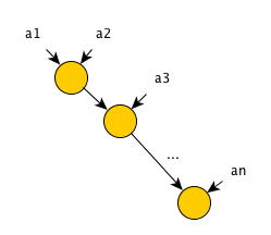
Obviously, for this algorithm, the number of operations is equal to the number of steps and is equal to n-1 = O (n) .
To “parallelize” the algorithm, it suffices to take into account the property of associativity of the convolution operator, and rearrange the parentheses in places: (... ((a ₁ * a ₂ ) * a ₃ ) ... * a _n ) = (a ₁ * a ₂ ) * ( a ₃ * a ₄ ) * ... * (a _n-1 * a _n ) . That is, we can in parallel calculate the values (a ₁ * a ₂ ) , (a ₃ * a ₄ ) and so on, and then perform a convolution operation on the resulting values. Execution tree for such an algorithm:

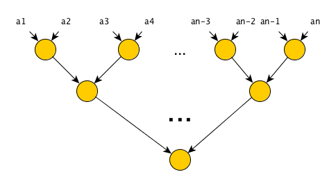
The number of steps is now equal to O (log (n)) , the number of operations is O (n) , which is good news — using a simple permutation of the parentheses, we obtained an algorithm with a significantly smaller number of steps, while the number of operations remained the same!
')

Scan

The scan operation is also performed on the array of elements, but is determined by the scan operator and the identity element . The scan operator must meet the same requirements as the convolution operator; the unit element must have the property I * a = a , where I is the unit element, * is the scan operator, and a is any other element. For example, for the addition operator, the unit element is 0, for the multiplication operator, 1. The result of applying the scan operation to the array of elements a ₁ , ..., a _n is an array of the same dimension n . There are two types of scanning operations:

1. Inclusive scanning - the result is calculated as: [reduce ([a ₁ ]), reduce ([a ₁ , a ₂ ]), ..., reduce ([a ₁ , ..., a _n ])) - in place i th input element in the output array will be the result of applying the convolution operation of all previous elements including the i- th element itself .
2. Exclusive scanning - the result is calculated as: [I, reduce ([a ₁ ]), ..., reduce ([a ₁ , ..., a _n-1 ])] - in place of the i -th input element in the output array there will be the result of applying the convolution operation of all previous elements excluding the i- th element itself - therefore the first element of the output array will be a single element.

The scanning operation is not so useful in itself, but it is one of the stages of many parallel algorithms. If you have an implementation at hand that only includes scanning, and you need an exclusive one - just pass the array [I, a ₁ , ..., a _n-1 ] instead of the array [a ₁ , ..., a _n ] ; if on the contrary, pass the array [a ₁ , ..., a _n , I] and remove the first element from the resulting array. Thus, both types of scanning are interchangeable. The execution tree of the sequential implementation of the scan operation will look the same as the convolution operation tree — just before each vertex of the tree we will write the current result of the convolution ( a ₁ before the first calculation for the inclusive scan and I for the exclusive) to the appropriate position of the output array.
Therefore, the number of steps and operations of such an algorithm will be equal to n − 1 = O (n) .
The easiest way to reduce the number of steps of the algorithm is fairly straightforward - since the scan operation is essentially determined by the convolution operation, what prevents us from simply starting the parallel version of the convolution operation n times? The number of steps in this case will indeed decrease - since all convolutions can be calculated independently, then the total number of steps is determined by the convolution with the largest number of steps - namely, the last one, which will be calculated on the entire input array. Total - O (log (n)) steps. However, the number of operations of such an algorithm is depressing - the first convolution will require 0 operations (not taking into account memory operations), the second - 1, ..., the last - n-1 operations, total - 1 + 2 + ... + n-1 = (n-1) * (n) / 2 = O (n ² ) .
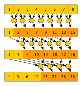
Consider 2 more efficient in terms of the number of operations of the algorithm for performing a scanning operation. The authors of the first algorithm - Daniel Hillis and Guy Steele, the algorithm is named after them - Hills & Steele scan. The algorithm is very simple, and can be written in 6 lines of python-pseudo-code:

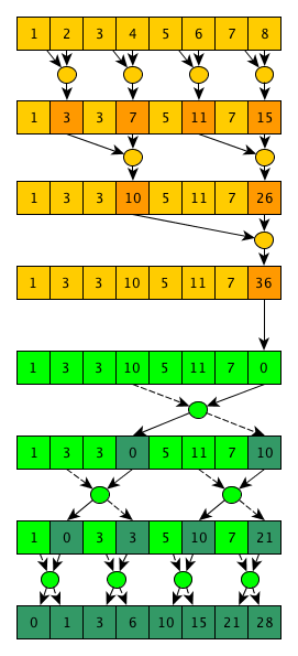
def hillie_steele_scan(io_arr): N = len(io_arr) for step in range(int(log(N, 2))+1): dist = 2**step for i in range(N-1, dist-1, -1): io_arr[i] = io_arr[i] + io_arr[i-dist] 

Or in words: starting from step 0 and ending with log ₂ (N) step (folding the fractional part), at each step step each element under the index i updates its value as a [i] = a [i] + a [i-2 ^step ] (naturally, if 2 ^step <= i ). If it is in mind to trace the execution of this algorithm for an array, it becomes clear why it is correct: after step 0, each element will contain the sum of itself and one adjacent element on the left; after step 1 - the sum of itself and 3 neighboring elements on the left ... at step n - the sum of itself and 2 ^{n + 1} -1 elements on the left - it is obvious that if the number of steps is equal to the integer part of log ₂ (N), then after the last step we will get an array corresponding to the operation of enabling scanning. From the description of the algorithm it is obvious that the number of steps is equal to log ₂ (N) + 1 = O (log (n)) . The number of operations is (N-1) + (N-2) + (N-4) ... + (N-2 ^{log ₂ (N)} ) = O (N * log (N)) . The execution tree of the algorithm on the example of an array of 8 elements and the sum operator looks like this:

The author of the second algorithm is Guy Blelloch, the algorithm is called (who would have thought) Blelloch scan. This algorithm implements exclusive scanning and is more complicated than the previous one, however, it requires fewer operations. The basic idea of ​​the algorithm is that if you look closely at the implementation of the parallel convolution algorithm, you can see that as we calculate the final value, we also calculate many useful intermediate values, for example, after the 1st step - the values a ₁ * a ₂ , a ₃ * a ₄ , ..., a _n-1 * a _n , after the 2nd step, the values ​​are a ₁ * a ₂ * a ₃ * a ₄ , a ₅ * a ₆ * a ₇ * a ₈ ... and etc. And if these values ​​are not discarded, then we can very quickly calculate, for example, the convolution of the first six elements - it is enough to take the already calculated convolution values ​​of the first 4 elements and elements a ₅ , a ₆ and “minimize” them. Therefore, the algorithm consists of 2 phases - in fact, the phase of convolution, and the second phase, called down-sweep (something like “scan down”). Graphically, the first phase looks like this (using the example of the same array of 8 elements and the sum operator):

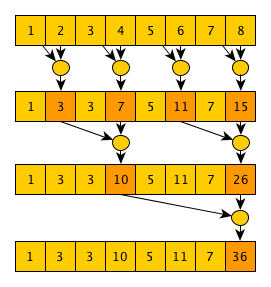
That is, practically the usual convolution algorithm, only intermediate convolutions, calculated over the elements a _i , a _{i + 1} , ..., a _{i + k,} replace the element a _{i + k} in the array.
The second phase is almost the mirror image of the first, but the “special” operator will be used, which returns 2 values, and at the beginning of the phase the last value of the array is replaced with a single element (0 for the addition operator):

This “special” operator takes 2 values ​​— left and right; in this case, it simply returns the right input as the left output, and the result of applying the scan operator to the left and right input values ​​as the right output. All these manipulations are needed in order to eventually minimize the calculated intermediate convolutions and get the desired result - eliminating scanning the input array. As is clearly seen from this illustration of the algorithm, the total number of operations is N-1 + N-1 + N-1 = O (N) , and the number of steps is 2 * log ₂ (N) = O (log (N)) . As usual, all that is good (improved asymptotics in this case) has to be paid - the algorithm is not only more complicated in pseudo-code, but also more difficult to implement effectively on the GPU - in the first steps of the algorithm we have quite a lot of work that can be done in parallel; when approaching the end of the first phase and at the beginning of the second phase, very little work will be done at each step; and at the end of the second phase, we will again have a lot of work at each step (by the way, several interesting parallel algorithms have this execution pattern). One of the possible solutions to this problem is to write 2 different cores - one will perform only one step, and be used at the beginning and at the end of the algorithm; the second will be designed to perform several steps in a row and will be used in the middle of execution - at the transition between phases. Well, on the host side it will be determined which kernel to call now, depending on the amount of work that needs to be done in the current step.

Histogram (histogram)

Informally, a histogram in the context of GPU programming (and not only) is the distribution of an array of elements over an array of cells, where each cell can contain only elements with certain properties. For example, having data on basketball players, such as height, weight, and so on. we want to know how many basketball players are <180 cm tall, from 180 cm to 190 cm and> 190 cm.
As usual, the sequential algorithm for computing the histogram is quite simple - just walk through all the elements in the array, and for each element, increase by 1 the value in the corresponding cell. The number of steps and operations is O (N) .
The simplest parallel histogram calculation algorithm is to run downstream to an array element, and each stream will increase the value in the cell only for its own element. Naturally, in this case it is necessary to use atomic operations. The disadvantage of this method is speed. Atomic operations force the threads to synchronize access to the cells and with an increase in the number of elements, the efficiency of this algorithm will fall.
One of the ways to avoid the use of atomic operations when building a histogram is to use a separate set of cells for each stream and the subsequent convolution of these local histograms. The disadvantage is that with a large number of threads we may simply not have enough memory to store all local histograms.
Another option to improve the efficiency of the simplest algorithm takes into account the specifics of CUDA, namely that we run threads in blocks that have common memory, and we can make a common histogram for all threads of one block, and add the same atomic operations to the end of the kernel this histogram to global. And although to build a common histogram of the block, it is still necessary to use atomic operations on the total memory of the block, they are much faster than atomic operations on global memory.

Conclusion

This part describes the basic primitives of many parallel algorithms. The practical implementation of most of these primitives will be shown in the next section, where we write bitwise sorting as an example.