Fourier transform in action: accurate signal frequency determination and note highlighting
latest article is available on makeloft.xyz
Let's start with the piano. Very simplified, this musical instrument is a set of white and black keys, when you click on each of which a certain sound of a predetermined frequency from low to high is extracted. Of course, each keyboard instrument has its own unique tonal color of the sound, thanks to which we can distinguish, for example, an accordion from a piano, but if roughly generalized, each key is simply a generator of sinusoidal acoustic waves of a certain frequency.
When a musician plays a composition, he alternately or simultaneously presses and releases the keys, as a result of which several sinusoidal signals overlap each other to form a drawing. This picture is perceived by us as a melody, so that we can easily recognize one work performed on various instruments in different genres or even unprofessionally sung by a person.
')
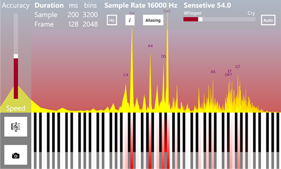
Graphic illustration of music pattern
Determination of frequency (guitar tuner mode)

The inverse problem is to disassemble the sounding musical composition into notes. That is, decompose the total acoustic signal caught by the ear into the original sinusoids. In essence, this process is a direct Fourier transform. And pressing the keys and extracting sound is a process of inverse Fourier transform.
Mathematically, in the first case, the decomposition of a complex periodic (on a certain time interval) function into a series of more elementary orthogonal functions (sinusoids and cosine curves) occurs. And in the second they are the inverse summation, that is, the synthesis of a complex signal.
Orthogonality, in some way, denotes immiscibility of functions. For example, if we take a few pieces of colored clay and glue them together, then we can still make out what colors were originally, but if we mix several jars of gouache paints well, then it will be impossible to restore the original colors without additional information.
(!) It is important to understand that when we undertake to analyze a real signal using the Fourier transform, we idealize the situation and assume that it is periodic in the current time interval and consists of elementary sinusoids . This is often the case, since acoustic signals, as a rule, are of a harmonic nature, but more complex cases are possible in general. Any of our assumptions about the nature of the signal usually lead to partial distortions and errors, but without this it is extremely difficult to isolate useful information from it.
Now we describe the whole process of analysis in more detail:
1. It all starts with the fact that sound waves oscillate the membrane of a microphone, which converts them into analog oscillations of electric current.
2. Then the analogue electrical signal is digitized. At this point it is worth staying in detail.
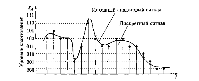
Since an analog signal mathematically consists of an infinite continuous in time set of amplitude point-values, in the measurement process we can extract from it only a finite series of values at discrete points in time, that is, in essence, perform time quantization ...
As a rule, sample values are taken at small equal time intervals, that is, with a certain frequency, for example, 16000 or 22000 Hz. However, in the general case, discrete readings can also be uneven, but this complicates the mathematical apparatus of analysis, therefore, in practice, it is usually not used.
There is an important Kotelnikov-Nyquist-Shannon theorem , which states that an analog periodic signal having a finite (limited in width) spectrum can be uniquely reconstructed without distortion and loss from its readings taken at a frequency greater than or equal to twice the upper frequency of the spectrum ( called sampling rate or Nyquist).
For this restoration, it is necessary to apply special interpolating functions, but the problem is that when using these functions, calculations must be performed on an infinite time interval, which is impossible in practice. Therefore, in real life it is impossible to arbitrarily increase the sampling rate artificially without distortion, even if it initially satisfies the Kotelnikov-Nyquist-Shannon theorem. For this operation apply filters Farrow.
Also, discretization occurs not only in time, but also in terms of the magnitude of the amplitude values, since the computer is able to manipulate only a limited set of numbers. This also introduces small errors.
3. At the next stage, the discrete direct Fourier transform occurs.
We select a short frame (interval) of the composition, consisting of discrete samples, which we conditionally consider periodic and apply the Fourier transform to it. As a result of the transformation, we obtain an array of complex numbers containing information about the amplitude and phase spectra of the frame being analyzed. Moreover, the spectra are also discrete with a step equal to (sampling frequency) / (number of samples). That is, the more samples we take, the more accurate the resolution is in frequency. However, with a constant sampling frequency, increasing the number of samples, we increase the analyzed time interval, and since in real music the notes have different sound durations and can quickly replace each other, they overlap, therefore the amplitude of long notes “eclipses” the amplitude of short notes. On the other hand, for guitar tuners this way of increasing the frequency resolution is well suited, since the note usually sounds long and alone.
There is also a fairly simple trick to increase the frequency resolution — you need to fill the original discrete signal with zeros between samples. However, as a result of this filling, the phase spectrum is strongly distorted, but the amplitude resolution increases. It is also possible to use Farrow filters and artificially increase the sampling rate, however, it also distorts the spectra.
The frame duration is usually about 30 ms to 1 s. The shorter it is, the better resolution we get in time, but the worst in frequency, the longer the sample, the better in frequency, but the worst in time. This is very similar to the Heisenberg uncertainty principle from quantum mechanics ... and is not simple, as Wikipedia says, the uncertainty relation in quantum mechanics in the mathematical sense is a direct consequence of the properties of the Fourier transform ...
It is also interesting that as a result of analyzing a single sinusoidal signal sample, the amplitude spectrum is very similar to the diffraction pattern ...
Sinusoidal signal bounded by a rectangular window and its "diffraction"
Light diffraction

In practice, this is an undesirable effect that complicates the analysis of signals, so they try to reduce it by applying window functions. A lot of such functions have been invented, below are the implementations of some of them, as well as a comparative impact on the spectrum of a single sinusoidal signal.
Applying a window function to an input frame is very simple:

As for computers, a fast Fourier transform algorithm was developed at the time, which minimizes the number of mathematical operations needed to calculate it. The only requirement of the algorithm is that the number of readings is a multiple of a power of two (256, 512, 1024, and so on).
Below is its classic recursive implementation in C #.
There are two types of FFT algorithms - with thinning in time and frequency, but both give identical results. The functions take an array of complex numbers filled with real values of the amplitudes of the signal in the time domain, and after their execution they return an array of complex numbers containing information about the amplitude and phase spectra. It is worth remembering that the real and imaginary parts of a complex number are not the same thing as its amplitude and phase!
magnitude = Math.Sqrt (x.Real * x.Real + x.Imaginary * x.Imaginary)
phase = Math.Atan2 (x.Imaginary, x.Real)
The resulting array of complex numbers is filled with exactly half of the useful information; the other half is only a mirror image of the first and can easily be excluded from consideration. If you think about it, this moment is well illustrated by the Kotelnikov-Nyquist-Shannon theorem, that the sampling frequency should not be less than the maximum doubled signal frequency ...
There is also a variation of the Cooley-Tukey FFT algorithm that is often used in practice, but it is a bit more difficult to understand.
Immediately after calculating the Fourier transform, it is convenient to normalize the amplitude spectrum:
This will lead to the fact that the magnitude of the amplitude values will be of the same order regardless of the size of the sample.
After calculating the amplitude and frequency spectra, it is easy to perform signal processing, for example, apply frequency filtering or compress. In essence, an equalizer can be made this way: by performing a direct Fourier transform, it is easy to increase or decrease the amplitude of a certain frequency range, and then perform the inverse Fourier transform (although the operation of real equalizers is usually based on a different principle — the phase shift of the signal). Yes, and compress the signal is very simple - you just need to make a dictionary, where the key is the frequency, and the value is the corresponding complex number. In the dictionary you need to enter only those frequencies, the amplitude of the signal which exceeds some minimum threshold. Information about "quiet" frequencies that are not heard by the ear will be lost, but you will get a noticeable compression while maintaining an acceptable sound quality. In part, this principle underlies many codecs.
4. Exact frequency determination
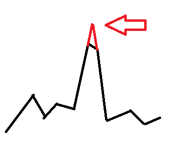
The discrete Fourier transform gives us a discrete spectrum, where each amplitude value is separated from its neighbors by equal intervals in frequency. And if the frequency in the signal is a multiple of the step equal to (sampling frequency) / (number of samples), then we will get a pronounced sharp peak, but if the signal frequency lies somewhere between the boundaries of the step closer to the middle, we will have a peak with a “cut off” peak and we it will be difficult to say what the frequency is. It may very well be that in the signal there are two frequencies lying next to each other. This is the limitation of the frequency resolution. Just as in a low-resolution photograph, small objects stick together and become indistinguishable, so also fine details of the spectrum can be lost.
But the frequencies of musical notes lie far from the grid of Fourier transform steps, but for everyday tasks of tuning musical instruments and recognizing notes, it is necessary to know the exact frequency. Moreover, at low octaves with a resolution of 1024 samples and below, the Fourier frequency grid becomes so rare that several notes start to fit in one step and it becomes virtually impossible to determine which one of them actually plays.
In order to somehow circumvent this limitation, approximating functions are sometimes used, for example, parabolic.
www.ingelec.uns.edu.ar/pds2803/Materiales/Articulos/AnalisisFrecuencial/04205098.pdf
mgasior.web.cern.ch/mgasior/pap/biw2004_poster.pdf
But all these are artificial measures that, improving some indicators, can give distortions in others.
Is there a more natural way to accurately determine the frequency?
Yes, and it is hidden just the same in using the phase spectrum of the signal, which is often neglected.
This method of signal frequency refinement is based on calculating the phase delay of the spectra of two frames superimposed on each other, but slightly shifted in time.
Read more about it on the links:
www.guitarpitchshifter.com/algorithm.html
www.dspdimension.com/admin/pitch-shifting-using-the-ft (+ code examples)
eudl.eu/pdf/10.1007/978-3-642-29157-9_43
ctuner.googlecode.com (examples of using the algorithm in C ++ and Java)
In C #, the implementation of the method looks quite simple:
The application is also simple:
Normally, the source frames are shifted by 1/16 or 1/32 of their length, that is, the ShiftsPerFrame is 16 or 32.
As a result, we obtain a frequency-amplitude dictionary, where the frequencies will be quite close to real. However, the "cut peaks" will still be observed, although less pronounced. To eliminate this disadvantage, you can simply "finish" them.
Perspectives
Music analysis of musical works opens up a number of interesting possibilities. After all, having a ready-made musical pattern available, you can search for other musical compositions with a similar pattern.
For example, one and the same work can be performed on another instrument, in a different manner, with a different timbre, or transposed in octaves, but the musical pattern will remain similar, which will allow you to find different versions of the performance of the same work. This is very similar to the game "guess the melody."
In some cases, such an analysis will help to identify plagiarism in musical works. Also, according to a musical pattern, theoretically, you can search for works of a particular mood or genre, which raises the search to a new level.
Results
This article outlines the basic principles for accurately determining the frequencies of acoustic signals and highlighting notes. And it also shows some subtle intuitive connection of the discrete Fourier transform with quantum physics, which pushes for reflection on a single picture of the world.
PS The Rainbow Framework (Rainbow Framework) containing all the above code examples can be downloaded from Codeplex .
PPS Perhaps this article will ever be very useful to you in your professional activity and will help save a lot of time and effort, so if you want to thank the author for your work, you can make a donation , buy an application ( free advertising version ), through which the article originated, or just express gratitude with a kind word.
Literature
1. Basic spectral analysis of sounds pandia.org/text/77/481/644.php
2. Algorithm Cooli-Tukey www.codeproject.com/Articles/32172/FFT-Guitar-Tuner
3. Resampling (resampling)
www.dsplib.ru/forum/viewtopic.php?f=5&t=11
www.dsplib.ru/content/farrow/farrow.html
4. Frequency correction by phase shift
www.guitarpitchshifter.com/algorithm.html
www.dspdimension.com/admin/pitch-shifting-using-the-ft (+ code examples)
eudl.eu/pdf/10.1007/978-3-642-29157-9_43
ctuner.googlecode.com (examples of using the algorithm in C ++ and Java)
Let's start with the piano. Very simplified, this musical instrument is a set of white and black keys, when you click on each of which a certain sound of a predetermined frequency from low to high is extracted. Of course, each keyboard instrument has its own unique tonal color of the sound, thanks to which we can distinguish, for example, an accordion from a piano, but if roughly generalized, each key is simply a generator of sinusoidal acoustic waves of a certain frequency.
When a musician plays a composition, he alternately or simultaneously presses and releases the keys, as a result of which several sinusoidal signals overlap each other to form a drawing. This picture is perceived by us as a melody, so that we can easily recognize one work performed on various instruments in different genres or even unprofessionally sung by a person.
')
Graphic illustration of music pattern
Determination of frequency (guitar tuner mode)
The inverse problem is to disassemble the sounding musical composition into notes. That is, decompose the total acoustic signal caught by the ear into the original sinusoids. In essence, this process is a direct Fourier transform. And pressing the keys and extracting sound is a process of inverse Fourier transform.
Mathematically, in the first case, the decomposition of a complex periodic (on a certain time interval) function into a series of more elementary orthogonal functions (sinusoids and cosine curves) occurs. And in the second they are the inverse summation, that is, the synthesis of a complex signal.
Orthogonality, in some way, denotes immiscibility of functions. For example, if we take a few pieces of colored clay and glue them together, then we can still make out what colors were originally, but if we mix several jars of gouache paints well, then it will be impossible to restore the original colors without additional information.
(!) It is important to understand that when we undertake to analyze a real signal using the Fourier transform, we idealize the situation and assume that it is periodic in the current time interval and consists of elementary sinusoids . This is often the case, since acoustic signals, as a rule, are of a harmonic nature, but more complex cases are possible in general. Any of our assumptions about the nature of the signal usually lead to partial distortions and errors, but without this it is extremely difficult to isolate useful information from it.
Now we describe the whole process of analysis in more detail:
1. It all starts with the fact that sound waves oscillate the membrane of a microphone, which converts them into analog oscillations of electric current.
2. Then the analogue electrical signal is digitized. At this point it is worth staying in detail.
Since an analog signal mathematically consists of an infinite continuous in time set of amplitude point-values, in the measurement process we can extract from it only a finite series of values at discrete points in time, that is, in essence, perform time quantization ...
As a rule, sample values are taken at small equal time intervals, that is, with a certain frequency, for example, 16000 or 22000 Hz. However, in the general case, discrete readings can also be uneven, but this complicates the mathematical apparatus of analysis, therefore, in practice, it is usually not used.
There is an important Kotelnikov-Nyquist-Shannon theorem , which states that an analog periodic signal having a finite (limited in width) spectrum can be uniquely reconstructed without distortion and loss from its readings taken at a frequency greater than or equal to twice the upper frequency of the spectrum ( called sampling rate or Nyquist).
For this restoration, it is necessary to apply special interpolating functions, but the problem is that when using these functions, calculations must be performed on an infinite time interval, which is impossible in practice. Therefore, in real life it is impossible to arbitrarily increase the sampling rate artificially without distortion, even if it initially satisfies the Kotelnikov-Nyquist-Shannon theorem. For this operation apply filters Farrow.
Also, discretization occurs not only in time, but also in terms of the magnitude of the amplitude values, since the computer is able to manipulate only a limited set of numbers. This also introduces small errors.
3. At the next stage, the discrete direct Fourier transform occurs.
We select a short frame (interval) of the composition, consisting of discrete samples, which we conditionally consider periodic and apply the Fourier transform to it. As a result of the transformation, we obtain an array of complex numbers containing information about the amplitude and phase spectra of the frame being analyzed. Moreover, the spectra are also discrete with a step equal to (sampling frequency) / (number of samples). That is, the more samples we take, the more accurate the resolution is in frequency. However, with a constant sampling frequency, increasing the number of samples, we increase the analyzed time interval, and since in real music the notes have different sound durations and can quickly replace each other, they overlap, therefore the amplitude of long notes “eclipses” the amplitude of short notes. On the other hand, for guitar tuners this way of increasing the frequency resolution is well suited, since the note usually sounds long and alone.
There is also a fairly simple trick to increase the frequency resolution — you need to fill the original discrete signal with zeros between samples. However, as a result of this filling, the phase spectrum is strongly distorted, but the amplitude resolution increases. It is also possible to use Farrow filters and artificially increase the sampling rate, however, it also distorts the spectra.
The frame duration is usually about 30 ms to 1 s. The shorter it is, the better resolution we get in time, but the worst in frequency, the longer the sample, the better in frequency, but the worst in time. This is very similar to the Heisenberg uncertainty principle from quantum mechanics ... and is not simple, as Wikipedia says, the uncertainty relation in quantum mechanics in the mathematical sense is a direct consequence of the properties of the Fourier transform ...
It is also interesting that as a result of analyzing a single sinusoidal signal sample, the amplitude spectrum is very similar to the diffraction pattern ...
Sinusoidal signal bounded by a rectangular window and its "diffraction"
Light diffraction
In practice, this is an undesirable effect that complicates the analysis of signals, so they try to reduce it by applying window functions. A lot of such functions have been invented, below are the implementations of some of them, as well as a comparative impact on the spectrum of a single sinusoidal signal.
Applying a window function to an input frame is very simple:
for (var i = 0; i < frameSize; i++) { frame[i] *= Window.Gausse(i, frameSize); } using System; using System.Numerics; namespace Rainbow { public class Window { private const double Q = 0.5; public static double Rectangle(double n, double frameSize) { return 1; } public static double Gausse(double n, double frameSize) { var a = (frameSize - 1)/2; var t = (n - a)/(Q*a); t = t*t; return Math.Exp(-t/2); } public static double Hamming(double n, double frameSize) { return 0.54 - 0.46*Math.Cos((2*Math.PI*n)/(frameSize - 1)); } public static double Hann(double n, double frameSize) { return 0.5*(1 - Math.Cos((2*Math.PI*n)/(frameSize - 1))); } public static double BlackmannHarris(double n, double frameSize) { return 0.35875 - (0.48829*Math.Cos((2*Math.PI*n)/(frameSize - 1))) + (0.14128*Math.Cos((4*Math.PI*n)/(frameSize - 1))) - (0.01168*Math.Cos((4*Math.PI*n)/(frameSize - 1))); } } } As for computers, a fast Fourier transform algorithm was developed at the time, which minimizes the number of mathematical operations needed to calculate it. The only requirement of the algorithm is that the number of readings is a multiple of a power of two (256, 512, 1024, and so on).
Below is its classic recursive implementation in C #.
using System; using System.Numerics; namespace Rainbow { public static class Butterfly { public const double SinglePi = Math.PI; public const double DoublePi = 2*Math.PI; public static Complex[] DecimationInTime(Complex[] frame, bool direct) { if (frame.Length == 1) return frame; var frameHalfSize = frame.Length >> 1; // frame.Length/2 var frameFullSize = frame.Length; var frameOdd = new Complex[frameHalfSize]; var frameEven = new Complex[frameHalfSize]; for (var i = 0; i < frameHalfSize; i++) { var j = i << 1; // i = 2*j; frameOdd[i] = frame[j + 1]; frameEven[i] = frame[j]; } var spectrumOdd = DecimationInTime(frameOdd, direct); var spectrumEven = DecimationInTime(frameEven, direct); var arg = direct ? -DoublePi/frameFullSize : DoublePi/frameFullSize; var omegaPowBase = new Complex(Math.Cos(arg), Math.Sin(arg)); var omega = Complex.One; var spectrum = new Complex[frameFullSize]; for (var j = 0; j < frameHalfSize; j++) { spectrum[j] = spectrumEven[j] + omega*spectrumOdd[j]; spectrum[j + frameHalfSize] = spectrumEven[j] - omega*spectrumOdd[j]; omega *= omegaPowBase; } return spectrum; } public static Complex[] DecimationInFrequency(Complex[] frame, bool direct) { if (frame.Length == 1) return frame; var halfSampleSize = frame.Length >> 1; // frame.Length/2 var fullSampleSize = frame.Length; var arg = direct ? -DoublePi/fullSampleSize : DoublePi/fullSampleSize; var omegaPowBase = new Complex(Math.Cos(arg), Math.Sin(arg)); var omega = Complex.One; var spectrum = new Complex[fullSampleSize]; for (var j = 0; j < halfSampleSize; j++) { spectrum[j] = frame[j] + frame[j + halfSampleSize]; spectrum[j + halfSampleSize] = omega*(frame[j] - frame[j + halfSampleSize]); omega *= omegaPowBase; } var yTop = new Complex[halfSampleSize]; var yBottom = new Complex[halfSampleSize]; for (var i = 0; i < halfSampleSize; i++) { yTop[i] = spectrum[i]; yBottom[i] = spectrum[i + halfSampleSize]; } yTop = DecimationInFrequency(yTop, direct); yBottom = DecimationInFrequency(yBottom, direct); for (var i = 0; i < halfSampleSize; i++) { var j = i << 1; // i = 2*j; spectrum[j] = yTop[i]; spectrum[j + 1] = yBottom[i]; } return spectrum; } } } There are two types of FFT algorithms - with thinning in time and frequency, but both give identical results. The functions take an array of complex numbers filled with real values of the amplitudes of the signal in the time domain, and after their execution they return an array of complex numbers containing information about the amplitude and phase spectra. It is worth remembering that the real and imaginary parts of a complex number are not the same thing as its amplitude and phase!
magnitude = Math.Sqrt (x.Real * x.Real + x.Imaginary * x.Imaginary)
phase = Math.Atan2 (x.Imaginary, x.Real)
The resulting array of complex numbers is filled with exactly half of the useful information; the other half is only a mirror image of the first and can easily be excluded from consideration. If you think about it, this moment is well illustrated by the Kotelnikov-Nyquist-Shannon theorem, that the sampling frequency should not be less than the maximum doubled signal frequency ...
There is also a variation of the Cooley-Tukey FFT algorithm that is often used in practice, but it is a bit more difficult to understand.
Immediately after calculating the Fourier transform, it is convenient to normalize the amplitude spectrum:
var spectrum = Butterfly.DecimationInTime(frame, true); for (var i = 0; i < frameSize; i++) { spectrum[i] /= frameSize; } This will lead to the fact that the magnitude of the amplitude values will be of the same order regardless of the size of the sample.
After calculating the amplitude and frequency spectra, it is easy to perform signal processing, for example, apply frequency filtering or compress. In essence, an equalizer can be made this way: by performing a direct Fourier transform, it is easy to increase or decrease the amplitude of a certain frequency range, and then perform the inverse Fourier transform (although the operation of real equalizers is usually based on a different principle — the phase shift of the signal). Yes, and compress the signal is very simple - you just need to make a dictionary, where the key is the frequency, and the value is the corresponding complex number. In the dictionary you need to enter only those frequencies, the amplitude of the signal which exceeds some minimum threshold. Information about "quiet" frequencies that are not heard by the ear will be lost, but you will get a noticeable compression while maintaining an acceptable sound quality. In part, this principle underlies many codecs.
4. Exact frequency determination
The discrete Fourier transform gives us a discrete spectrum, where each amplitude value is separated from its neighbors by equal intervals in frequency. And if the frequency in the signal is a multiple of the step equal to (sampling frequency) / (number of samples), then we will get a pronounced sharp peak, but if the signal frequency lies somewhere between the boundaries of the step closer to the middle, we will have a peak with a “cut off” peak and we it will be difficult to say what the frequency is. It may very well be that in the signal there are two frequencies lying next to each other. This is the limitation of the frequency resolution. Just as in a low-resolution photograph, small objects stick together and become indistinguishable, so also fine details of the spectrum can be lost.
But the frequencies of musical notes lie far from the grid of Fourier transform steps, but for everyday tasks of tuning musical instruments and recognizing notes, it is necessary to know the exact frequency. Moreover, at low octaves with a resolution of 1024 samples and below, the Fourier frequency grid becomes so rare that several notes start to fit in one step and it becomes virtually impossible to determine which one of them actually plays.
In order to somehow circumvent this limitation, approximating functions are sometimes used, for example, parabolic.
www.ingelec.uns.edu.ar/pds2803/Materiales/Articulos/AnalisisFrecuencial/04205098.pdf
mgasior.web.cern.ch/mgasior/pap/biw2004_poster.pdf
But all these are artificial measures that, improving some indicators, can give distortions in others.
Is there a more natural way to accurately determine the frequency?
Yes, and it is hidden just the same in using the phase spectrum of the signal, which is often neglected.
This method of signal frequency refinement is based on calculating the phase delay of the spectra of two frames superimposed on each other, but slightly shifted in time.
Read more about it on the links:
www.guitarpitchshifter.com/algorithm.html
www.dspdimension.com/admin/pitch-shifting-using-the-ft (+ code examples)
eudl.eu/pdf/10.1007/978-3-642-29157-9_43
ctuner.googlecode.com (examples of using the algorithm in C ++ and Java)
In C #, the implementation of the method looks quite simple:
using System; using System.Collections.Generic; using System.Linq; using System.Numerics; namespace Rainbow { // Δ∂ωπ public static class Filters { public const double SinglePi = Math.PI; public const double DoublePi = 2*Math.PI; public static Dictionary<double, double> GetJoinedSpectrum( IList<Complex> spectrum0, IList<Complex> spectrum1, double shiftsPerFrame, double sampleRate) { var frameSize = spectrum0.Count; var frameTime = frameSize/sampleRate; var shiftTime = frameTime/shiftsPerFrame; var binToFrequancy = sampleRate/frameSize; var dictionary = new Dictionary<double, double>(); for (var bin = 0; bin < frameSize; bin++) { var omegaExpected = DoublePi*(bin*binToFrequancy); // ω=2πf var omegaActual = (spectrum1[bin].Phase - spectrum0[bin].Phase)/shiftTime; // ω=∂φ/∂t var omegaDelta = Align(omegaActual - omegaExpected, DoublePi); // Δω=(∂ω + π)%2π - π var binDelta = omegaDelta/(DoublePi*binToFrequancy); var frequancyActual = (bin + binDelta)*binToFrequancy; var magnitude = spectrum1[bin].Magnitude + spectrum0[bin].Magnitude; dictionary.Add(frequancyActual, magnitude*(0.5 + Math.Abs(binDelta))); } return dictionary; } public static double Align(double angle, double period) { var qpd = (int) (angle/period); if (qpd >= 0) qpd += qpd & 1; else qpd -= qpd & 1; angle -= period*qpd; return angle; } } } The application is also simple:
var spectrum0 = Butterfly.DecimationInTime(frame0, true); var spectrum1 = Butterfly.DecimationInTime(frame1, true); for (var i = 0; i < frameSize; i++) { spectrum0[i] /= frameSize; spectrum1[i] /= frameSize; } var spectrum = Filters.GetJoinedSpectrum(spectrum0, spectrum1, ShiftsPerFrame, Device.SampleRate); Normally, the source frames are shifted by 1/16 or 1/32 of their length, that is, the ShiftsPerFrame is 16 or 32.
As a result, we obtain a frequency-amplitude dictionary, where the frequencies will be quite close to real. However, the "cut peaks" will still be observed, although less pronounced. To eliminate this disadvantage, you can simply "finish" them.
using System; using System.Collections.Generic; using System.Linq; using System.Numerics; namespace Rainbow { public static class Filters { public static Dictionary<double, double> Antialiasing(Dictionary<double, double> spectrum) { var result = new Dictionary<double, double>(); var data = spectrum.ToList(); for (var j = 0; j < spectrum.Count - 4; j++) { var i = j; var x0 = data[i].Key; var x1 = data[i + 1].Key; var y0 = data[i].Value; var y1 = data[i + 1].Value; var a = (y1 - y0)/(x1 - x0); var b = y0 - a*x0; i += 2; var u0 = data[i].Key; var u1 = data[i + 1].Key; var v0 = data[i].Value; var v1 = data[i + 1].Value; var c = (v1 - v0)/(u1 - u0); var d = v0 - c*u0; var x = (d - b)/(a - c); var y = (a*d - b*c)/(a - c); if (y > y0 && y > y1 && y > v0 && y > v1 && x > x0 && x > x1 && x < u0 && x < u1) { result.Add(x1, y1); result.Add(x, y); } else { result.Add(x1, y1); } } return result; } } } Perspectives
Music analysis of musical works opens up a number of interesting possibilities. After all, having a ready-made musical pattern available, you can search for other musical compositions with a similar pattern.
For example, one and the same work can be performed on another instrument, in a different manner, with a different timbre, or transposed in octaves, but the musical pattern will remain similar, which will allow you to find different versions of the performance of the same work. This is very similar to the game "guess the melody."
In some cases, such an analysis will help to identify plagiarism in musical works. Also, according to a musical pattern, theoretically, you can search for works of a particular mood or genre, which raises the search to a new level.
Results
This article outlines the basic principles for accurately determining the frequencies of acoustic signals and highlighting notes. And it also shows some subtle intuitive connection of the discrete Fourier transform with quantum physics, which pushes for reflection on a single picture of the world.
PS The Rainbow Framework (Rainbow Framework) containing all the above code examples can be downloaded from Codeplex .
PPS Perhaps this article will ever be very useful to you in your professional activity and will help save a lot of time and effort, so if you want to thank the author for your work, you can make a donation , buy an application ( free advertising version ), through which the article originated, or just express gratitude with a kind word.
Literature
1. Basic spectral analysis of sounds pandia.org/text/77/481/644.php
2. Algorithm Cooli-Tukey www.codeproject.com/Articles/32172/FFT-Guitar-Tuner
3. Resampling (resampling)
www.dsplib.ru/forum/viewtopic.php?f=5&t=11
www.dsplib.ru/content/farrow/farrow.html
4. Frequency correction by phase shift
www.guitarpitchshifter.com/algorithm.html
www.dspdimension.com/admin/pitch-shifting-using-the-ft (+ code examples)
eudl.eu/pdf/10.1007/978-3-642-29157-9_43
ctuner.googlecode.com (examples of using the algorithm in C ++ and Java)
Source: https://habr.com/ru/post/247385/
All Articles