Interpolation: draw smooth graphs using Bezier curves

Good day, harbilitator.

In this article I would like to tell you about a once thought-out algorithm (or, most likely, a re-invented bicycle) of building a smooth graph at given points using Bezier curves. The article was written under the influence of this article here and a very useful comment from comrade lany , for which a special thank you to them.

Formulation of the problem
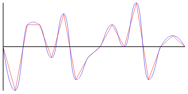
There is an array of Y-cov points located evenly along the X-axis. It is necessary to get a smooth graph that passes through all given points. The example in the figure below:
')


All who are interested, please under the cat.

There are a number of standard solutions for carrying out a smooth curve through points (for this reason many interesting things are written in the article already mentioned ), such as, for example, interpolation by splines. When this algorithm was invented in the third year, the word “interpolation” terrified me, and googling at the request “smoothing of graphs” did not give a reasonable understanding of the results. But somehow I reached the Bezier curves and I really liked them. Draws fast, the algorithm is intuitive ... What else is needed for happiness. Well, somehow it started.

main idea

Split the idea into three subparagraphs to make it clearer and more readable.

1. Bezier curves are well written on the wiki and javascript.ru . If you read carefully, you can pay attention that the Bezier curve goes out from the first point tangent to the straight start-point-first_-stop_point. Similarly, and at the end - the curve comes with respect to a straight line last_thatt-end-point. Thus, it turns out that if we have one curve end at point A and go tangently to line a , and the other curve leaves this point A tangently to that same line a , then this transition between two Bezier curves will turn out smooth.
2. Proceeding from the first point, it turns out that our points of support on the left and right of point A must lie on one straight line. After thinking a bit, it was decided that this line should be such that ∠BAB ₁ = ∠CAC ₁ (figure below), where the points B ₁ and C ₁ are reference points.
   
   
   
   
   
3. The distance from point A to point B ₁ and C ₁ was decided to be equal to half the step in X between points B and A , A and C , etc. It is difficult for me to somehow substantiate such a choice, but it is important that this distance be less than the X step between points A and B , otherwise it may result in something like the figure below. It is important to understand that the longer this distance is, the more winding the curve will be and vice versa. Half a step in X seems to be optimal, but options are already possible here.
   
   
   
   
   

Thus, it turns out that the task is reduced to finding a straight line ( B ₁ C ₁ ) and, in fact, reference points B ₁ and C ₁ , from which we will later build Bezier curves.

Search straight

As is known, a straight line on a plane is expressed by the formula y = kx + b , where k is the tangent of the angle of inclination of the straight line to the X axis, and b is the “height” of the intersection of the straight line and the Y axis.

K factor search

I will say in advance that k = tg (φ) = tg ((α-β) / 2) = (Sqrt (((Y _A -Y _B ) ² + ΔX ² ) * ((Y _A- Y _C ) ² + ΔX ² )) - ΔX ² - (Y _A -Y _B ) * (Y _A -Y _C )) / (ΔX * (Y _C -Y _B )) , where ΔX is the distance along X between the points of the graph (I remind you that us points are evenly spaced on X). Below is a mathematical proof of the correctness of the formula, but if you are not in the mood, you can simply skip it.



And so, k we found. Looking ahead to say that b is not useful to us in the calculations. Let's start the search for reference points.

Looking for pivot points

Immediately I will say that: ΔX '= ΔX / 2 * Sqrt (1 / (1 + k ² )) , the coordinates of the reference point on the right: X _C1 = X _A + ΔX'; Y _C1 = Y _A + k * ΔX ' , and on the left: X _B1 = X _A -ΔX'; Y _B1 = Y _A -k * ΔX ' .

To enjoy!

1. From comrade lany (a huge thank you to him and plus him to karma), I learned that html5 using the quadraticCurveTo () and bezierCurveTo () functions can draw bezier curves on the canvas. Accordingly, the algorithm can be applied with JavaScript.
2. A nice feature of the algorithm is that the graph predictably “protrudes” beyond the boundaries of the space of points through which we actually plot. If we take the distance to the reference points equal to half of the step in X (the [AC ₁ ] segment in the last figure), then a gap of a quarter of the step in X above and below the canvas boundaries will suffice.

JSFiddle implementation example


UPDATE:

1. Attempts to make the pivot points have to be counted once, and then, when scaling the graph, simply using their coordinates, failed. It all comes down to the fact that the calculation of the coefficient k includes the current scale in X, and the current scale in Y. And to pull them out of the formula does not go. Comrade quverty warned me about it and turned out to be right.
2. I would like to note that the curvature of the plotted graph can be adjusted. To do this, change the distance to the reference points - change the coefficient ΔX '= ΔX / 2 * Sqrt (1 / (1 + k ² )) , namely - the denominator of this piece of it: ΔX / 2 . The denominator less than 1 should not be taken (read the third subparagraph of the paragraph "Basic idea"). You can experiment on JSFiddle (line 129 of JavaScript).
3. Pay attention to the implementation of the spline Catmulla-Roma comrade IIvana . And thank him for this comment.