Scapegoat trees

Today we look at a data structure called a scapegoat tree. “Scapegoat”, who does not know, is translated as “scapegoat”, which makes the literal translation of the structure name strange, therefore we will use the original name. Search trees, as you may know, there are so many different types, and all of them are based on the same idea: " But it would be good to search through an element not all the data in a row, but only some part, preferably size log (N) order ".

To do this, each vertex stores references to its children and some criterion according to which when searching it is clear which of the child vertices should be passed to. For logarithmic time, this will all work when the tree is balanced (well, or tends to it) - i.e. when the “height” of each of the subtrees of each vertex is about the same. But the ways of balancing a tree are already in each type of tree: in the red and black trees in the tops are stored “color” markers, telling when and how to rebalance the tree, in AVL-trees in the tops the difference in children's heights is kept, Splay-trees for balancing are forced change the tree during search operations, etc.

Scapegoat-tree also has its own approach to solving the problem of balancing a tree. As for all other cases, it is not perfect, but it is quite applicable in some situations.
')
The advantages of Scapegoat-tree include:

• No need to store any additional data in the vertices (which means we win by memory from the red-black, AVL and Cartesian trees)
• No need to rebalance the tree during the search operation (which means we can guarantee the maximum search time O (log N), unlike Splay-trees, where only damp O (log N) is guaranteed)
• The amortized complexity of insertion and deletion of O (log N) is in general similar to other types of trees.
• When building a tree, we choose a certain coefficient of “rigor” α, which allows us to “tune” the tree, making the search operations faster by slowing down the modification operations or vice versa. You can implement the data structure, and then select the coefficient by the results of tests on real data and the specific use of the tree.

The disadvantages include:

• In the worst case, tree modification operations can take O (n) time (they still have O (log N) amortized complexity, but there is no protection from "bad" cases).
• You can incorrectly estimate the frequency of different operations with a tree and make a mistake with the choice of the coefficient α - as a result, often used operations will work long and rarely used - quickly, which is somehow not good.

Let's understand what a Scapegoat tree is and how to perform search, insert and delete operations for it.

The concepts used (the square brackets in the notation above mean that we store this value explicitly, which means we can take O (1) time. The parentheses mean that the value will be calculated along the way, that is, the memory is not consumed, but time to calculate)

• T - so we will denote a tree
• root [T] - the root of the tree T
• left [x] - left "son" of the top x
• right [x] - right "son" of vertex x
• brother (x) - brother of vertex x (the vertex that has a common parent with x)
• depth (x) is the depth of vertex x. This is the distance from it to the root (the number of edges)
• height (T) is the depth of the tree T. This is the depth of the deepest tip of the tree T
• size (x) is the weight of vertex x. This is the number of all its child vertices + 1 (she herself)
• size [T] is the size of the tree T. This is the number of vertices in it (root weight)

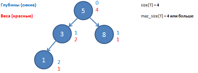
Now we introduce the concepts we need for a Scapegoat tree:

• max_size [T] - the maximum size of the tree. This is the maximum value that the size [T] parameter has taken since the last rebalancing. If rebalancing has just occurred, then max_size [T] = size [T]
• The coefficient α is a number in the range of [0.5; 1), determining the required degree of quality of balancing the tree. Some vertex x is called “α-balanced in weight,” if the weight of her left son is less than or equal to α * size (x) and the weight of her right son is less than or equal to α * size (x).
  
  size (left [x]) ≤ α * size (x)
  size (right [x]) ≤ α * size (x)
  

Let's try to understand this criterion. If α = 0.5, we require that in the left subtree there are exactly as many vertices as in the right one (± 1). Those. in fact, this requirement is a perfectly balanced tree. With α> 0.5 we say “ok, let the balancing be not perfect, let one of the subtrees be allowed to have more peaks than the other”. When α = 0.6, one of the subtrees of x can contain up to 60% of all the vertices of the subtree x so that x is still considered “α-balanced in weight”. It is easy to see that for α tending to 1, we actually agree to consider even the usual coherent list to be “α-balanced in weight”.

Now let's see how the usual operations are performed in the Scapegoat tree.
At the beginning of working with a tree, we choose the parameter α in the range [0.5; one). Also, we set up two variables to store the current values ​​of size [T] and max_size [T] and reset them.

Search
So, we have some Scapegoat-tree and we want to find an element in it. Since this is a binary search tree, then the search will be standard: go from the root, compare the top with the desired value, if found - return, if the value at the top is less - recursively search in the left subtree, if more - in the right. The tree during the search is not modified.

The complexity of the search operation, as you might have guessed, depends on α and is expressed by the formula

Those. the complexity is, of course, logarithmic, only the base of the logarithm is interesting. When α is close to 0.5, we get the binary (or almost binary) logarithm, which means the ideal (or almost perfect) search speed. If α is close to one, the base of the logarithm tends to one, and therefore the total complexity tends to O (N). Yeah, and no one promised the ideal.

Insert
The insertion of a new element into the Scapegoat-tree is a classic: with a search we are looking for a place to hang a new vertex, well, we hang it up. It is easy to understand that this action could disrupt α-balancing by weight for one or more tree nodes. And now begins what gave the name to the data structure: we are looking for a “scapegoat” (Scapegoat-vertex) —the vertex for which α-balance is lost and its subtree must be rebuilt. The vertex just inserted itself, although it is to blame for the loss of balance, cannot become a scapegoat - it has no “children” yet, which means its balance is perfect. Accordingly, you need to go through the tree from this top to the root, counting the weights for each top along the way. If there is a vertex on this path, for which the criterion of α-balance by weight is violated, we completely rearrange the corresponding subtree to restore α-balance by weight.

Along the way, a number of questions arise:
- And how to get from the top "up" to the root? Do we need to keep references to parents?
- Not. Since we came to the place of insertion of a new vertex from the root of the tree - we have a stack, which is all the way from the root to the new vertex. We take parents from it.

- And how to calculate the "weight" of the top - we do not store it at the very top?
- No, we do not store. For a new vertex, weight = 1. For its parent, weight = 1 (weight of new vertex) + 1 (weight of the parent itself) + size (brother (x)).

- Well, ok, but how to count size (brother (x))?
- recursively. Yes, it will take O (size (brother (x))) time. Realizing that in the worst case, we may have to calculate the weight of half a tree - we see the very complexity O (N) in the worst case, which was mentioned at the beginning. But since we are going around the subtree of an α-balanced tree by weight, it can be shown that the amortized complexity of the operation will not exceed O (log N).

“ But there may be several peaks for which the α-balance is broken - what to do?”
- Short answer: you can choose any. Long answer: in the original document with a description of the data structure, there are a couple of heuristics, how can you choose “a specific scapegoat” (this is the terminology that went!), But in general they boil down to “so we tried it this way and that, experiments showed that This is better, but we cannot explain why. ”

- And how to rebalance the found Scapegoat-tops?
- There are two ways: trivial and slightly more cunning.

Trivial rebalancing

1. We go around the entire subtree of the Scapegoat-vertex (including itself) with the help of in-order traversal - at the output we get a sorted list (property In-order traversal of the binary search tree).
2. We find the median on this segment, suspend it as the root of the subtree.
3. For the “left” and “right” subtree, we repeat the same operation recursively.

It can be seen that the whole thing requires O (size (Scapegoat-vertex)) time and the same amount of memory.

Slightly more clever rebalancing

We are unlikely to improve the rebalancing time - after all, each vertex must be “hung” to a new place. But we can try to save memory. Let's look at the "trivial" algorithm more closely. Here we choose the median, hang it to the root, the tree is divided into two subtrees - and it is divided very clearly. No one can choose "some other median" or suspend the "right" subtree instead of the left one. The same uniqueness follows us in each of the following steps. Those. for some list of vertices sorted in ascending order, we will have exactly one tree generated by the algorithm. And where did we get the sorted list of vertices? From in-order traversal of the original tree. Those. each vertex found in the in-order traversal of the rebalancing tree corresponds to one specific position in the new tree. And we can calculate this position in principle without creating the most sorted list. And having calculated - immediately write it there. There is only one problem - we are overwriting with some kind of (perhaps not yet viewed) peak - what to do? Store it. Where? Well, allocate for the list of such peaks memory. But this memory will no longer need O (size (N)), but only O (log N).

As an exercise, imagine in your mind a tree consisting of three peaks — a root and two pendants as “left” sons of peaks. In-order traversal will return these vertices to us in order from the deepest to the root, but we will only have one vertex (the deepest) to store in a separate memory, because when we arrive at the second vertex we will already know that this is the median and it will be the root, and the other two peaks will be its children. Those. the memory consumption here is for the storage of one vertex, which is consistent with the upper estimate for a tree of three vertices - log (3).

Remove vertex
We delete the vertex by simply deleting the vertex of the binary search tree (search, deletion, possible re-hanging of children).
Next, check the condition
size [T] <α * max_size [T]
if it is executed, the tree could lose α-balancing by weight, which means it is necessary to perform a complete rebalancing of the tree (starting from the root) and assign max_size [T] = size [T]

How is it all productive?

The lack of an overhead projector for memory and rebalancing in the search is good, it works for us. On the other hand, rebalancing with modifications is not so very cheap. Well, the choice of α significantly affects the performance of certain operations. The inventors themselves compared the performance of a Scapegoat tree to red-black and Splay trees. They managed to choose α in such a way that, on random data, the Scapegoat tree surpassed all other types of trees in speed on any operations (which is actually quite good). Unfortunately, on a monotonically increasing data set, the Scapegoat tree works worse in terms of insert operations and it did not work for any α for winning Scapegoat.