Processing NBA data for 30 years using MongoDB Aggregation
Note Trans.: American writer Michael Lewis is known not only for his stories about Wall Street traders , but also (first of all) for the Moneyball book, after which the film with the same name (“The Man Who Changed Everything”) was later shot. Its main character, Billie Bean, general manager of the baseball team Oakland Athleticks, creates a competitive team based solely on an analysis of the players' statistics.
Bearing in mind this, we decided to publish one interesting material about how interesting and nontrivial conclusions can be reached by analyzing the publicly available statistics of NBA games over the past 30 years using the MongoDB Aggregation framework. Despite the fact that in this example, the author analyzes the performance of teams as a whole, rather than the statistics for individual players (it is also publicly available), he comes to very interesting conclusions - based on his calculations, it’s quite possible to carry out an independent analysis, at one time the heroes of Moneyball arrived.
')
When searching for a tool for analyzing large data sets and complex structures, you can instinctively refer to Hadoop. On the other hand, if you store your data in MongoDB, using the Hadoop Connector seems unnecessary, especially if all your data is stored on a laptop. Fortunately, the built-in framework MongoDB Aggregation offers a quick solution for conducting complex analytics directly from a MongoDB instance without installing additional software.
Being a basketball fan since childhood, I always dreamed of learning how to conduct comprehensive analytics of NBA statistics. When the time came for the MongoDB Driver Days hackathon, and the leading Ruby-engineer Gary Murakami offered to compile an interesting array of data, we sat down and ran and started the scraper from noon to evening. scraper, a program to extract data from web pages] for the site basketball-reference.com. The resulting dataset consisted of the final score and player statistics for each match of the NBA regular season starting from the 1985–1986 season.
The documentation for the aggregation frameworks [data] often uses arrays of postcode data that demonstrate how to use such a framework. However, the processing of data on the population of the United States is not very impressive to my imagination, and there are certain formats for using the aggregation framework that cannot be illustrated with an example of an array of postal codes. I hope this dataset allows you to take a fresh look at the aggregation framework, and you will like to understand the NBA statistics. You can download the dataset here and insert it into your MongoDB instance using the mongorestore command.
First, let's look at the data structure. Since the 1985–86 season, 31,686 games have been played in the NBA regular season. Each individual document is information about a single game. Below are the metadata for the 1985-86 season opening match between the Washington Bullets and Atlanta Hawks teams, as shown in RoboMongo, MongoDB’s universal graphical user interface:

The document includes an embedded subsection with detailed match statistics, a date field, and information about the teams that played. You can see that “Bullets” won on the road with a score of 100-91. The match statistics data (box score) are similarly divided by teams in the array, starting with the winning one. Note that the “won” flag is an element of the high-level box score object along with the “team” and “players” elements.
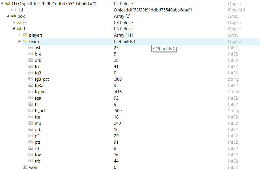
Further, the game statistics is divided into team statistics and player statistics. The statistics of the team in the figure above displays the general data for the team Atlanta Hawks, according to which they realized 41 of 92 shots from the game and scored only 9 of 18 goals from the penalty line. The dataset of the players contains the same information, but distributed among individual players. For example, below you will see that the star “Hawks” Dominic Wilkins scored 32 points with 15 successful shots from the game of 29 and recorded 3 interceptions.

In a general sense, the MongoDB Aggregation framework is implemented as an aggregate shell function: it contains a set of operations that can be chained. Each stage in the chain of operations is carried out on the basis of the results of the previous stage, and at each stage it is possible to form a sample and return the result as a document.
Before starting a serious calculation, I propose to launch a simple test of the system’s performance and calculate the 5 teams with the most victories in the 1999-2000 season. These commands can be determined by following the chain of operations from 6 stages:
The final shell command is presented below. This command on my laptop runs in real time even when there are no indexes in the database, since there are only 31,686 documents in the sample.
This simple example can be summarized to answer the question of which team won the most wins in the period between the seasons 2000-2001 and 2009-2010, replacing at the step of using the $ match function the time for playing games for the period between August 1, 2000 and August 1, 2010. It turns out that San Antonio Spurs won 579 victories in this period, beating Dallas Mavericks a little with 568 victories.
Now we’ll do something a little more interesting using a couple of aggregation operators that you rarely see when analyzing data sets of postcodes: the $ gte operator and the $ cond operator at the $ project stage . We use these operators in order to calculate how often the team, which made more selections in defense than their opponents, wins over the entire data array.
A slight difficulty arises here when finding the difference in the total number of rebounds in defending the winning and losing teams. The aggregation framework calculates this difference a bit ambiguously, but using the $ cond operator, we can convert the document so that the total number of rebounds in the defense will be negative if the team lost. In this case, we will be able to use the $ group operator to calculate the difference of rebounds in defense in each game. Let's go through the algorithm in stages:
The result was rather curious: the team, which recorded more rebounds in defense, won 75% of cases. For comparison, a team that scores more shots from the game than the other team wins only 78.8% of cases! Try rewriting the aggregation algorithm for other indicators, such as throws from the game, three-pointers, the number of losses, etc. You will get a number of rather interesting results. The number of rebounds in the attack, as it turns out, should not be used to predict the outcome of the game, since the team that took more rebounds in the attack, won only 51% of cases. It turns out that by the number of three-point shots the winner can be predicted much more precisely: the team with a large number of three-point shots won 64% of the time.
Let's analyze the data for which it will be interesting to draw a graph. We will calculate the percentage of team wins as a function of the number of rebounds implemented in defense. This aggregation is fairly easy to do: all you need to do is execute the $ unwind operator for match statistics and use $ group to calculate the average number of won flags for all values of the total number of rebounds in defense.
If you visualize the results of the aggregation, you can get a good schedule, clearly showing a fairly high correlation between the number of rebounds in defense and the percentage of wins. A curious fact: the team that picked up the fewest rebounds in the event of a victory was Toronto Raptors in the 1995–96 season, beating Milwaukee Bucks with a score of 93–87 on December 26, 1995, despite only 14 rebounds in the defense made in this game.

In order to conduct a similar analysis for the total number of rebounds as compared to the rebounds in defense, we can quite easily change the aggregation algorithm above and see if the result changes.
And he really is changing! Somewhere after the result of the 53 total selections, the positive correlation between the total number of rebounds and the percentage of wins disappears completely! The correlation here is clearly not as high as in the case of rebounds in defense. Incidentally, Cleveland Cavaliers took over New York Knicks with a score of 101-97 on April 11, 1996, despite the fact that in general they took only 21 rebounds. On the other hand, San Antonio Spurs lost to Houston Rockets with a score of 112-110 on January 4, 1992, while their total number of rebounds was 75.
I hope this post has interested you in the topic of aggregation frameworks just like me. Let me remind you once again that you can download the dataset here - I strongly recommend that you work with this data yourself.
Bearing in mind this, we decided to publish one interesting material about how interesting and nontrivial conclusions can be reached by analyzing the publicly available statistics of NBA games over the past 30 years using the MongoDB Aggregation framework. Despite the fact that in this example, the author analyzes the performance of teams as a whole, rather than the statistics for individual players (it is also publicly available), he comes to very interesting conclusions - based on his calculations, it’s quite possible to carry out an independent analysis, at one time the heroes of Moneyball arrived.
')
When searching for a tool for analyzing large data sets and complex structures, you can instinctively refer to Hadoop. On the other hand, if you store your data in MongoDB, using the Hadoop Connector seems unnecessary, especially if all your data is stored on a laptop. Fortunately, the built-in framework MongoDB Aggregation offers a quick solution for conducting complex analytics directly from a MongoDB instance without installing additional software.
Being a basketball fan since childhood, I always dreamed of learning how to conduct comprehensive analytics of NBA statistics. When the time came for the MongoDB Driver Days hackathon, and the leading Ruby-engineer Gary Murakami offered to compile an interesting array of data, we sat down and ran and started the scraper from noon to evening. scraper, a program to extract data from web pages] for the site basketball-reference.com. The resulting dataset consisted of the final score and player statistics for each match of the NBA regular season starting from the 1985–1986 season.
The documentation for the aggregation frameworks [data] often uses arrays of postcode data that demonstrate how to use such a framework. However, the processing of data on the population of the United States is not very impressive to my imagination, and there are certain formats for using the aggregation framework that cannot be illustrated with an example of an array of postal codes. I hope this dataset allows you to take a fresh look at the aggregation framework, and you will like to understand the NBA statistics. You can download the dataset here and insert it into your MongoDB instance using the mongorestore command.
Examine the data
First, let's look at the data structure. Since the 1985–86 season, 31,686 games have been played in the NBA regular season. Each individual document is information about a single game. Below are the metadata for the 1985-86 season opening match between the Washington Bullets and Atlanta Hawks teams, as shown in RoboMongo, MongoDB’s universal graphical user interface:
The document includes an embedded subsection with detailed match statistics, a date field, and information about the teams that played. You can see that “Bullets” won on the road with a score of 100-91. The match statistics data (box score) are similarly divided by teams in the array, starting with the winning one. Note that the “won” flag is an element of the high-level box score object along with the “team” and “players” elements.
Further, the game statistics is divided into team statistics and player statistics. The statistics of the team in the figure above displays the general data for the team Atlanta Hawks, according to which they realized 41 of 92 shots from the game and scored only 9 of 18 goals from the penalty line. The dataset of the players contains the same information, but distributed among individual players. For example, below you will see that the star “Hawks” Dominic Wilkins scored 32 points with 15 successful shots from the game of 29 and recorded 3 interceptions.
Conducting aggregation
In a general sense, the MongoDB Aggregation framework is implemented as an aggregate shell function: it contains a set of operations that can be chained. Each stage in the chain of operations is carried out on the basis of the results of the previous stage, and at each stage it is possible to form a sample and return the result as a document.
Before starting a serious calculation, I propose to launch a simple test of the system’s performance and calculate the 5 teams with the most victories in the 1999-2000 season. These commands can be determined by following the chain of operations from 6 stages:
- We use the $ match operator to work only with games that took place between August 1, 1999 and August 1, 2000 — two dates that are far enough away from any of the NBA games and reliably limit this season.
- We use the $ unwind operator to generate one document for each team in the match.
- Again, we use the $ match operator to weed out only the winning teams.
- Use the $ group operator to calculate how many times this command appears as a result in step 3.
- Use the $ sort operator to sort the number of wins in descending order.
- We use the $ limit operator to select the 5 teams with the highest number of wins.
The final shell command is presented below. This command on my laptop runs in real time even when there are no indexes in the database, since there are only 31,686 documents in the sample.
db.games.aggregate([ { $match : { date : { $gt : ISODate("1999-08-01T00:00:00Z"), $lt : ISODate("2000-08-01T00:00:00Z") } } }, { $unwind : '$teams' }, { $match : { 'teams.won' : 1 } }, { $group : { _id : '$teams.name', wins : { $sum : 1 } } }, { $sort : { wins : -1 } }, { $limit : 5 } ]); This simple example can be summarized to answer the question of which team won the most wins in the period between the seasons 2000-2001 and 2009-2010, replacing at the step of using the $ match function the time for playing games for the period between August 1, 2000 and August 1, 2010. It turns out that San Antonio Spurs won 579 victories in this period, beating Dallas Mavericks a little with 568 victories.
db.games.aggregate([ { $match : { date : { $gt : ISODate("2000-08-01T00:00:00Z"), $lt : ISODate("2010-08-01T00:00:00Z") } } }, { $unwind : '$teams' }, { $match : { 'teams.won' : 1 } }, { $group : { _id : '$teams.name', wins : { $sum : 1 } } }, { $sort : { wins : -1 } }, { $limit : 5 } ]); Determining the relationship of statistics with the number of wins
Now we’ll do something a little more interesting using a couple of aggregation operators that you rarely see when analyzing data sets of postcodes: the $ gte operator and the $ cond operator at the $ project stage . We use these operators in order to calculate how often the team, which made more selections in defense than their opponents, wins over the entire data array.
A slight difficulty arises here when finding the difference in the total number of rebounds in defending the winning and losing teams. The aggregation framework calculates this difference a bit ambiguously, but using the $ cond operator, we can convert the document so that the total number of rebounds in the defense will be negative if the team lost. In this case, we will be able to use the $ group operator to calculate the difference of rebounds in defense in each game. Let's go through the algorithm in stages:
- We use the $ unwind operator to get a document with detailed statistics for each team in this game.
- We use the $ project and $ cond operators to convert each document, so that the total number of team selections in defense will be negative if it lost: information about the game results is determined by the “won” checkbox.
- We use the $ group and $ sum operators to calculate the total number of rebounds in each game. Since, as a result of the previous stage, the total number of rebounds of the losing team has become negative, now in each document there is a difference between the number of rebounds in defending the winning and losing teams.
- We use the $ project and $ gte operators to create a document that will contain the winningTeamHigher flag, which is true, if the winning team has made more defense selections than the losing one.
- We use the $ group and $ sum operators in order to calculate how many games the winningTeamHigher flag takes on the value "true".
db.games.aggregate([ { $unwind : '$box' }, { $project : { _id : '$_id', stat : { $cond : [ { $gt : ['$box.won', 0] }, '$box.team.drb', { $multiply : ['$box.team.drb', -1] } ] } } }, { $group : { _id : '$_id', stat : { $sum : '$stat' } } }, { $project : { _id : '$_id', winningTeamHigher : { $gte : ['$stat', 0] } } }, { $group : { _id : '$winningTeamHigher', count : { $sum : 1 } } } ]); The result was rather curious: the team, which recorded more rebounds in defense, won 75% of cases. For comparison, a team that scores more shots from the game than the other team wins only 78.8% of cases! Try rewriting the aggregation algorithm for other indicators, such as throws from the game, three-pointers, the number of losses, etc. You will get a number of rather interesting results. The number of rebounds in the attack, as it turns out, should not be used to predict the outcome of the game, since the team that took more rebounds in the attack, won only 51% of cases. It turns out that by the number of three-point shots the winner can be predicted much more precisely: the team with a large number of three-point shots won 64% of the time.
We match the rebounds in defense and the total number of rebounds with the winning percentage.
Let's analyze the data for which it will be interesting to draw a graph. We will calculate the percentage of team wins as a function of the number of rebounds implemented in defense. This aggregation is fairly easy to do: all you need to do is execute the $ unwind operator for match statistics and use $ group to calculate the average number of won flags for all values of the total number of rebounds in defense.
db.games.aggregate([ { $unwind : '$box' }, { $group : { _id : '$box.team.drb', winPercentage : { $avg : '$box.won' } } }, { $sort : { _id : 1 } } ]); If you visualize the results of the aggregation, you can get a good schedule, clearly showing a fairly high correlation between the number of rebounds in defense and the percentage of wins. A curious fact: the team that picked up the fewest rebounds in the event of a victory was Toronto Raptors in the 1995–96 season, beating Milwaukee Bucks with a score of 93–87 on December 26, 1995, despite only 14 rebounds in the defense made in this game.
In order to conduct a similar analysis for the total number of rebounds as compared to the rebounds in defense, we can quite easily change the aggregation algorithm above and see if the result changes.
db.games.aggregate([ { $unwind : '$box' }, { $group : { _id : '$box.team.trb', winPercentage : { $avg : '$box.won' } } }, { $sort : { _id : 1 } } ]); And he really is changing! Somewhere after the result of the 53 total selections, the positive correlation between the total number of rebounds and the percentage of wins disappears completely! The correlation here is clearly not as high as in the case of rebounds in defense. Incidentally, Cleveland Cavaliers took over New York Knicks with a score of 101-97 on April 11, 1996, despite the fact that in general they took only 21 rebounds. On the other hand, San Antonio Spurs lost to Houston Rockets with a score of 112-110 on January 4, 1992, while their total number of rebounds was 75.
Conclusion
I hope this post has interested you in the topic of aggregation frameworks just like me. Let me remind you once again that you can download the dataset here - I strongly recommend that you work with this data yourself.
Source: https://habr.com/ru/post/246317/
All Articles