Hacker's guide to neural networks. Schemes of real values. Patterns in the "reverse" stream. Example "One neuron"
Content:
Let's look again at our example of a scheme with numbers entered. The first diagram shows us the "raw" values, and the second - the gradients that return to their original values, as discussed earlier. Note that the gradient always reduces to +1. This is the standard push for the scheme in which the value should increase.
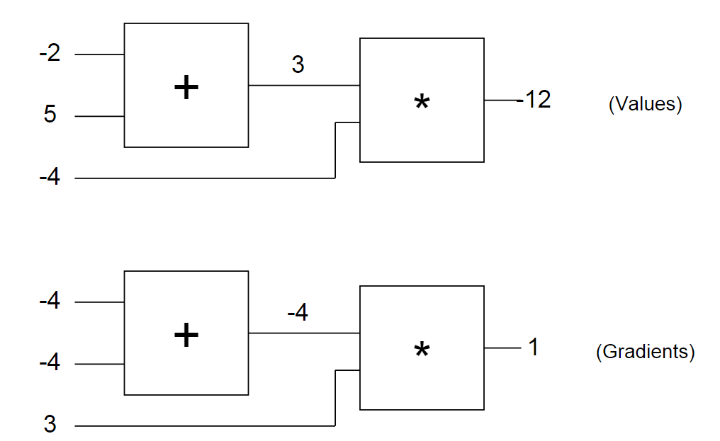
After a while, you will begin to notice patterns in how gradients are returned in a pattern. For example, the logical element + always raises the gradient and simply passes it to all the original values (note that in the example with -4 it was simply transferred to both the original values of the logical element +). This is because its own derivative for the original values is +1, regardless of what the actual values of the original data are equal to, so in the chain rule, the gradient from the top is simply multiplied by 1 and remains the same.
')
The same happens, for example, with the logical element max (x, y). Since the gradient of the element max (x, y) with respect to its initial values is +1 for that value of x or y, which is greater, and 0 for the second, this logical element in the process of inverse error distribution is effectively used only as a “switch” gradient: it takes the gradient from the top and “directs” it to its original value, which is higher when going back.
Numeric gradient check
Before we finish with this section, let's just make sure that the analytical gradient we calculated for the back propagation of error is correct. Let's remember that we can do this by simply calculating a numerical gradient, and making sure we get [-4, -4, 3] for x, y, z. Here is the code:
Example: One neuron
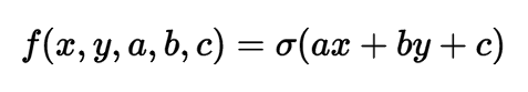
In the previous section, you finally understood the concept of back propagation of an error. Let us now consider a more complex and practical example. We consider a two-dimensional neuron that calculates the following function:
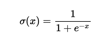
In this expression, σ is a sigmoid function. It can be described as a “compressing function”, since it takes the original value and compresses it so that it is between zero and one: Extremely negative values are compressed towards zero, and positive values are compressed towards one. For example, we have the expression sig (-5) = 0.006, sig (0) = 0.5, sig (5) = 0.993. Sigmoid function is defined as follows:
The gradient with respect to its only initial value, as indicated in Wikipedia (or, if you know the calculation methods, you can calculate it yourself), looks like the following expression:
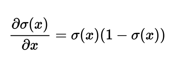
For example, if the initial value of the sigmoid logic element is x = 3, the logical element will calculate the result of the equation f = 1.0 / (1.0 + Math.exp (-x)) = 0.95, after which the (local) gradient will have the following view: dx = (0.95) * (1 - 0.95) = 0.0475.
That's all we need to use this logical element: we know how to take the original value and move it through the sigmoid logical element, and we also have an expression for the gradient relative to its original value, so we can also perform the inverse distribution mistakes with it. Another point to which you should pay attention - technically, the sigmoid function consists of a whole set of logical elements arranged in a row that calculate additional atomic functions: the logical element of exponentiation, addition and division. This attitude works fine, but for this example I decided to compress all these logical elements to one, which computes the sigmoid at a time, since the gradient expression turned out to be quite simple.
Let's take this opportunity to carefully structure the associated code in a convenient, modular way. To begin with, I would like to draw your attention to the fact that each line in our graphs has two numbers connected with it:
1. The value that it has in the direct passage
2. Gradient (i.e. push), which passes back along it while going back
Let's create a simple segment structure (Unit) that will store these two values along each line. Our logical elements will not work on top of segments: they will take them as initial values and create them as output values.
In addition to segments, we also need three logical elements: +, * and sig (sigmoid). Let's start by applying the logical element of multiplication. Here I use Javascript, which interestingly simulates classes using functions. If you are not familiar with Javascript, what happens here is the definition of a class that has certain properties (accessed using the this keyword), and some methods (which are placed in the function prototype in Javascript). Just remember them as class methods. Also do not forget that the way we will use them is that we first send (forward) all the logical elements one by one, and then we return them back (backward) in the reverse order. Here is the implementation of this:
The multiplication logic element takes two segments, each of which contains a value, and creates a segment that stores its result. Gradient is assigned zero as initial value. Then note that when we call the backward function, we get the gradient from the result of the segment that we created during the front pass (which I hope will now have a filled gradient) and multiply it by the local gradient for this logical element (a chain rule! ). This logical element performs multiplication (u0.value * u1.value) in the front pass, so we recall that the gradient with respect to u0 is equal to u1.value and with respect to u1 is equal to u0.value. Also note that we use + = to add to the gradient with the backward function. This may allow us to use the result of one logical element several times (imagine it as a branching line), since it turns out that the gradients along these branches are simply summed up when calculating the final gradient with respect to the result of the circuit. The remaining two logical elements are defined in the same way:
Note, again, that the backward function in all cases simply calculates the local derivative with respect to its initial value, after which it multiplies it by the gradient from the segment above (ie, the chain rule is valid). To determine everything in full, let's finally write out the forward and reverse flows for our two-dimensional neuron with some approximate values:
Now let's calculate the gradient: just repeat everything in the reverse order and call the backward function! We recall that we saved the pointers to the segments when we were passing forward, so the logical element has access to its original values, as well as to the output segment that it had previously created.
Notice that the first line sets the output gradient (the most recent segment) to 1.0 to trigger the gradient chain. This can be interpreted as a push on the last logical element with a force equal to +1. In other words, we are pulling the whole circuit, forcing it to apply forces that will increase the output value. If we did not set it to 1, all gradients would be calculated as zero due to multiplication according to the chain rule. Finally, let's make the initial values respond to the calculated gradients and check that the function has increased:
Success! 0.8825 higher than the previous value, 0.8808. Finally, let's check that we correctly did backward propagation of the error by checking the numerical gradient:
Thus, all this gives the same values as the gradients of the back propagation error [-0.105, 0.315, 0.105, 0.105, 0.210]. Fine!
I hope you understand that even though we only looked at an example with one neuron, the code I gave above is a fairly simple way to calculate the gradients of arbitrary expressions (including very deep expressions). All you need to do is write small logic elements that will calculate local simple derivatives with respect to their initial values, link them to a graph, run forward to calculate the output value, and then perform a reverse pass that will connect the gradient across path to the original value.
Let's look again at our example of a scheme with numbers entered. The first diagram shows us the "raw" values, and the second - the gradients that return to their original values, as discussed earlier. Note that the gradient always reduces to +1. This is the standard push for the scheme in which the value should increase.
After a while, you will begin to notice patterns in how gradients are returned in a pattern. For example, the logical element + always raises the gradient and simply passes it to all the original values (note that in the example with -4 it was simply transferred to both the original values of the logical element +). This is because its own derivative for the original values is +1, regardless of what the actual values of the original data are equal to, so in the chain rule, the gradient from the top is simply multiplied by 1 and remains the same.
')
The same happens, for example, with the logical element max (x, y). Since the gradient of the element max (x, y) with respect to its initial values is +1 for that value of x or y, which is greater, and 0 for the second, this logical element in the process of inverse error distribution is effectively used only as a “switch” gradient: it takes the gradient from the top and “directs” it to its original value, which is higher when going back.
Numeric gradient check
Before we finish with this section, let's just make sure that the analytical gradient we calculated for the back propagation of error is correct. Let's remember that we can do this by simply calculating a numerical gradient, and making sure we get [-4, -4, 3] for x, y, z. Here is the code:
// var x = -2, y = 5, z = -4; // var h = 0.0001; var x_derivative = (forwardCircuit(x+h,y,z) - forwardCircuit(x,y,z)) / h; // -4 var y_derivative = (forwardCircuit(x,y+h,z) - forwardCircuit(x,y,z)) / h; // -4 var z_derivative = (forwardCircuit(x,y,z+h) - forwardCircuit(x,y,z)) / h; // 3 Example: One neuron
In the previous section, you finally understood the concept of back propagation of an error. Let us now consider a more complex and practical example. We consider a two-dimensional neuron that calculates the following function:
In this expression, σ is a sigmoid function. It can be described as a “compressing function”, since it takes the original value and compresses it so that it is between zero and one: Extremely negative values are compressed towards zero, and positive values are compressed towards one. For example, we have the expression sig (-5) = 0.006, sig (0) = 0.5, sig (5) = 0.993. Sigmoid function is defined as follows:
The gradient with respect to its only initial value, as indicated in Wikipedia (or, if you know the calculation methods, you can calculate it yourself), looks like the following expression:
For example, if the initial value of the sigmoid logic element is x = 3, the logical element will calculate the result of the equation f = 1.0 / (1.0 + Math.exp (-x)) = 0.95, after which the (local) gradient will have the following view: dx = (0.95) * (1 - 0.95) = 0.0475.
That's all we need to use this logical element: we know how to take the original value and move it through the sigmoid logical element, and we also have an expression for the gradient relative to its original value, so we can also perform the inverse distribution mistakes with it. Another point to which you should pay attention - technically, the sigmoid function consists of a whole set of logical elements arranged in a row that calculate additional atomic functions: the logical element of exponentiation, addition and division. This attitude works fine, but for this example I decided to compress all these logical elements to one, which computes the sigmoid at a time, since the gradient expression turned out to be quite simple.
Let's take this opportunity to carefully structure the associated code in a convenient, modular way. To begin with, I would like to draw your attention to the fact that each line in our graphs has two numbers connected with it:
1. The value that it has in the direct passage
2. Gradient (i.e. push), which passes back along it while going back
Let's create a simple segment structure (Unit) that will store these two values along each line. Our logical elements will not work on top of segments: they will take them as initial values and create them as output values.
// var Unit = function(value, grad) { // , this.value = value; // , this.grad = grad; } In addition to segments, we also need three logical elements: +, * and sig (sigmoid). Let's start by applying the logical element of multiplication. Here I use Javascript, which interestingly simulates classes using functions. If you are not familiar with Javascript, what happens here is the definition of a class that has certain properties (accessed using the this keyword), and some methods (which are placed in the function prototype in Javascript). Just remember them as class methods. Also do not forget that the way we will use them is that we first send (forward) all the logical elements one by one, and then we return them back (backward) in the reverse order. Here is the implementation of this:
var multiplyGate = function(){ }; multiplyGate.prototype = { forward: function(u0, u1) { // u0 u1 utop this.u0 = u0; this.u1 = u1; this.utop = new Unit(u0.value * u1.value, 0.0); return this.utop; }, backward: function() { // // , // . this.u0.grad += this.u1.value * this.utop.grad; this.u1.grad += this.u0.value * this.utop.grad; } } The multiplication logic element takes two segments, each of which contains a value, and creates a segment that stores its result. Gradient is assigned zero as initial value. Then note that when we call the backward function, we get the gradient from the result of the segment that we created during the front pass (which I hope will now have a filled gradient) and multiply it by the local gradient for this logical element (a chain rule! ). This logical element performs multiplication (u0.value * u1.value) in the front pass, so we recall that the gradient with respect to u0 is equal to u1.value and with respect to u1 is equal to u0.value. Also note that we use + = to add to the gradient with the backward function. This may allow us to use the result of one logical element several times (imagine it as a branching line), since it turns out that the gradients along these branches are simply summed up when calculating the final gradient with respect to the result of the circuit. The remaining two logical elements are defined in the same way:
var addGate = function(){ }; addGate.prototype = { forward: function(u0, u1) { this.u0 = u0; this.u1 = u1; // this.utop = new Unit(u0.value + u1.value, 0.0); return this.utop; }, backward: function() { // . 1 this.u0.grad += 1 * this.utop.grad; this.u1.grad += 1 * this.utop.grad; } } var sigmoidGate = function() { // this.sig = function(x) { return 1 / (1 + Math.exp(-x)); }; }; sigmoidGate.prototype = { forward: function(u0) { this.u0 = u0; this.utop = new Unit(this.sig(this.u0.value), 0.0); return this.utop; }, backward: function() { var s = this.sig(this.u0.value); this.u0.grad += (s * (1 - s)) * this.utop.grad; } } Note, again, that the backward function in all cases simply calculates the local derivative with respect to its initial value, after which it multiplies it by the gradient from the segment above (ie, the chain rule is valid). To determine everything in full, let's finally write out the forward and reverse flows for our two-dimensional neuron with some approximate values:
// var a = new Unit(1.0, 0.0); var b = new Unit(2.0, 0.0); var c = new Unit(-3.0, 0.0); var x = new Unit(-1.0, 0.0); var y = new Unit(3.0, 0.0); // var mulg0 = new multiplyGate(); var mulg1 = new multiplyGate(); var addg0 = new addGate(); var addg1 = new addGate(); var sg0 = new sigmoidGate(); // var forwardNeuron = function() { ax = mulg0.forward(a, x); // a*x = -1 by = mulg1.forward(b, y); // b*y = 6 axpby = addg0.forward(ax, by); // a*x + b*y = 5 axpbypc = addg1.forward(axpby, c); // a*x + b*y + c = 2 s = sg0.forward(axpbypc); // sig(a*x + b*y + c) = 0.8808 }; forwardNeuron(); console.log('circuit output: ' + s.value); // 0.8808 Now let's calculate the gradient: just repeat everything in the reverse order and call the backward function! We recall that we saved the pointers to the segments when we were passing forward, so the logical element has access to its original values, as well as to the output segment that it had previously created.
s.grad = 1.0; sg0.backward(); // axpbypc addg1.backward(); // axpby c addg0.backward(); // ax by mulg1.backward(); // b y mulg0.backward(); // a x Notice that the first line sets the output gradient (the most recent segment) to 1.0 to trigger the gradient chain. This can be interpreted as a push on the last logical element with a force equal to +1. In other words, we are pulling the whole circuit, forcing it to apply forces that will increase the output value. If we did not set it to 1, all gradients would be calculated as zero due to multiplication according to the chain rule. Finally, let's make the initial values respond to the calculated gradients and check that the function has increased:
var step_size = 0.01; a.value += step_size * a.grad; // a.grad -0.105 b.value += step_size * b.grad; // b.grad 0.315 c.value += step_size * c.grad; // c.grad 0.105 x.value += step_size * x.grad; // x.grad 0.105 y.value += step_size * y.grad; // y.grad 0.210 forwardNeuron(); console.log('circuit output after one backprop: ' + s.value); // 0.8825 Success! 0.8825 higher than the previous value, 0.8808. Finally, let's check that we correctly did backward propagation of the error by checking the numerical gradient:
var forwardCircuitFast = function(a,b,c,x,y) { return 1/(1 + Math.exp( - (a*x + b*y + c))); }; var a = 1, b = 2, c = -3, x = -1, y = 3; var h = 0.0001; var a_grad = (forwardCircuitFast(a+h,b,c,x,y) - forwardCircuitFast(a,b,c,x,y))/h; var b_grad = (forwardCircuitFast(a,b+h,c,x,y) - forwardCircuitFast(a,b,c,x,y))/h; var c_grad = (forwardCircuitFast(a,b,c+h,x,y) - forwardCircuitFast(a,b,c,x,y))/h; var x_grad = (forwardCircuitFast(a,b,c,x+h,y) - forwardCircuitFast(a,b,c,x,y))/h; var y_grad = (forwardCircuitFast(a,b,c,x,y+h) - forwardCircuitFast(a,b,c,x,y))/h; Thus, all this gives the same values as the gradients of the back propagation error [-0.105, 0.315, 0.105, 0.105, 0.210]. Fine!
I hope you understand that even though we only looked at an example with one neuron, the code I gave above is a fairly simple way to calculate the gradients of arbitrary expressions (including very deep expressions). All you need to do is write small logic elements that will calculate local simple derivatives with respect to their initial values, link them to a graph, run forward to calculate the output value, and then perform a reverse pass that will connect the gradient across path to the original value.
Source: https://habr.com/ru/post/246093/
All Articles