Comparing the speed of building linear models in R and Eviews
If you need to evaluate an econometric model with a small number of observations, the software in which this can be done is determined solely by your preferences and financial capabilities. But if the number of observations is large? Regression is not always evaluated in one instant. In this post, I compare the time estimates of linear regression in R and Eviews depending on the number of observations.
To perform this test, we will use simple linear regression:
y i = 10 + 5x i + ε i
The number of observations in the regression N will change and compare the evaluation time for each. I took N from 100,000 to 10,000,000 in increments of 100,000.
')
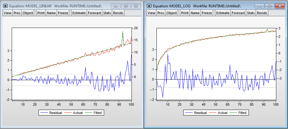
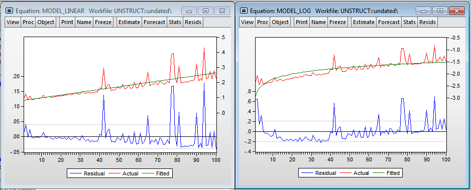
I added the variable dum - dummy to one of the observations (you can see the outburst on the chart, at that moment I needed to open the browser). As expected, the number of observations has a significant effect on the regression construction time. The multiplicative model gives more beautiful results. There is even a hint of normality of residuals in the regression. Using the linear model, we get that each additional million observations increases the construction time by 1.39 seconds, and the model in logarithms shows the elasticity of the number of observations over time 1.014 (i.e., if the number of observations increases by 1%, then the time for calculating the regression will increase by 1.014%) .
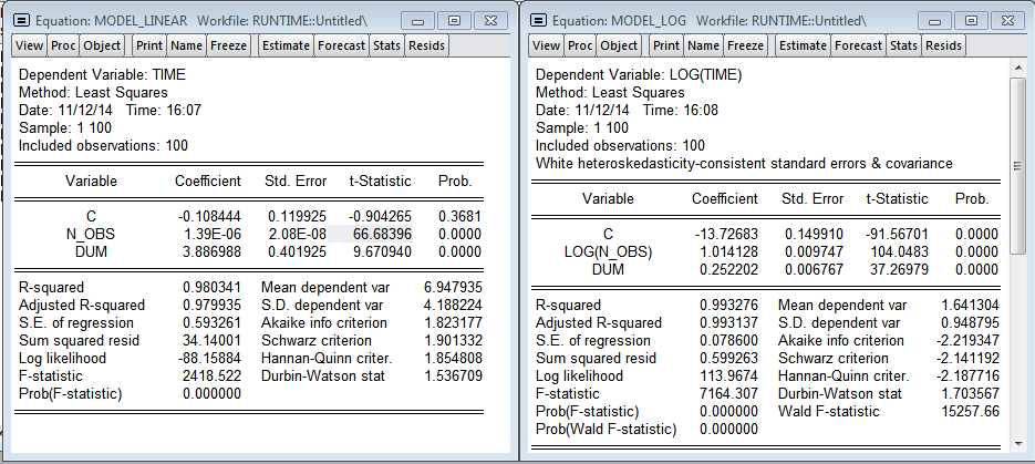
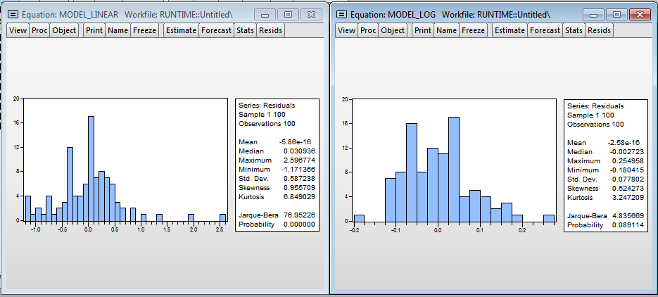
Visually, histograms of model residuals are not similar to the normal distribution, and therefore the estimates obtained in the models are biased, because, most likely, we do not take into account a significant variable - the level of processor utilization. Nevertheless, in the logarithmic model one can accept the hypothesis of normality (since the critical value of the test statistics of Harkey-Beer is 8.9% and exceeds the standard critical level of significance of 5%).
The models obtained in Eviews do not qualitatively describe the dependence of the construction time on the number of observations. The linear model predicts that an additional million observations will increase the model estimation time by 0.018 seconds (75.8 times less than in R). In the logarithmic model, the elasticity is 0.306 (3.3 times less than in R)
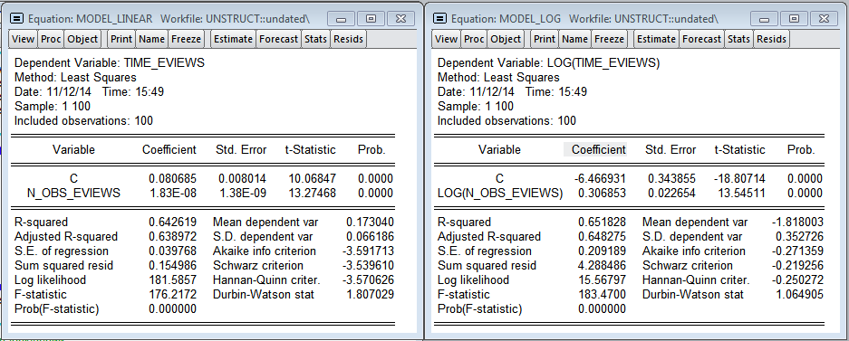
The graphs show a significant amount of emissions, which most likely indicates a much more significant effect of the processor load on the calculation time in Eviews. There is heteroscedasticity in errors, which argues in favor of the inclusion of a variable — the level of processor utilization in the model. It should be noted that Eviews practically does not consume RAM, while R cumulatively increases the amount of memory consumed for its needs and does not release it until the program is closed.
Again, the residuals in the models are not normal, you need to add more variables.
In the end I want to say that you should not immediately write it in R as a minus. It is possible that such a different calculation time turned out because the lm () function that I used in R creates a large object of type lm which contains a lot of information about the evaluated model and for 100,000 observations already weighs about 23 Mb, which is again stored in random access memory. If you are interested, you can repeat a similar test using any other functions from R or, for example, implement a gradient descent algorithm, which can be found here .
To perform this test, we will use simple linear regression:
y i = 10 + 5x i + ε i
The number of observations in the regression N will change and compare the evaluation time for each. I took N from 100,000 to 10,000,000 in increments of 100,000.
')
What came out of it
Results R (Linear and logarithmic models)
I added the variable dum - dummy to one of the observations (you can see the outburst on the chart, at that moment I needed to open the browser). As expected, the number of observations has a significant effect on the regression construction time. The multiplicative model gives more beautiful results. There is even a hint of normality of residuals in the regression. Using the linear model, we get that each additional million observations increases the construction time by 1.39 seconds, and the model in logarithms shows the elasticity of the number of observations over time 1.014 (i.e., if the number of observations increases by 1%, then the time for calculating the regression will increase by 1.014%) .
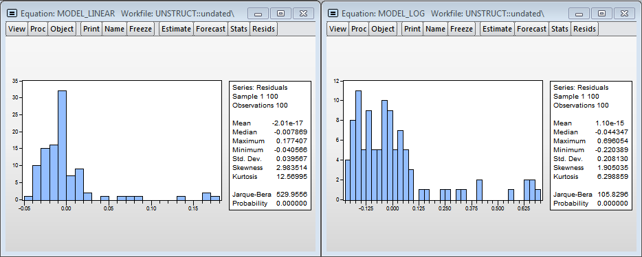
Residual histograms
Visually, histograms of model residuals are not similar to the normal distribution, and therefore the estimates obtained in the models are biased, because, most likely, we do not take into account a significant variable - the level of processor utilization. Nevertheless, in the logarithmic model one can accept the hypothesis of normality (since the critical value of the test statistics of Harkey-Beer is 8.9% and exceeds the standard critical level of significance of 5%).
Eviews Results (Linear and Logarithmic Models)
The models obtained in Eviews do not qualitatively describe the dependence of the construction time on the number of observations. The linear model predicts that an additional million observations will increase the model estimation time by 0.018 seconds (75.8 times less than in R). In the logarithmic model, the elasticity is 0.306 (3.3 times less than in R)
The graphs show a significant amount of emissions, which most likely indicates a much more significant effect of the processor load on the calculation time in Eviews. There is heteroscedasticity in errors, which argues in favor of the inclusion of a variable — the level of processor utilization in the model. It should be noted that Eviews practically does not consume RAM, while R cumulatively increases the amount of memory consumed for its needs and does not release it until the program is closed.
Again, the residuals in the models are not normal, you need to add more variables.
In the end I want to say that you should not immediately write it in R as a minus. It is possible that such a different calculation time turned out because the lm () function that I used in R creates a large object of type lm which contains a lot of information about the evaluated model and for 100,000 observations already weighs about 23 Mb, which is again stored in random access memory. If you are interested, you can repeat a similar test using any other functions from R or, for example, implement a gradient descent algorithm, which can be found here .
Code in R
library(ggplot2) # , - N <- seq(100000,10000000, by = 100000) time.vector <- rep(0,length(N)) # - N count = 1 for (n in N) { X <- matrix(c(rep(1,n),seq(1:n)),ncol = 2) y <- matrix(X[, 1] * 10 + 5 * X[, 2] + rnorm(n,0,1)) t <- Sys.time() lm1 <- lm(y ~ 0 + X) t1 <- Sys.time() lm1.time <- t1 - t time.vector[count] <- lm1.time count <- count + 1 } # times <- data.frame(N,time.vector) names(times) <- c('N_obs','Time') ggplot(data = times, aes(N_obs, Time, size = 2)) + geom_point() write.csv(times,'times.csv') Eviews code
' workfile, - wfcreate(wf=unstruct, page=undated) u 10000000 scalar time_elapsed = 0 series time_eviews = 0 series n_obs_eviews = 0 ' , R, - , for !n = 1 to 100 smpl @first @first + !n * 100000 - 1 series trend = @trend+1 series y = 10 + 5 * trend + nrnd tic equation eq1.ls yc trend time_elapsed = @toc smpl @first + !n - 1 @first + !n - 1 time_eviews = time_elapsed n_obs_eviews = !n * 100000 next smpl @first @first + 99 ' - equation model_linear.ls time_eviews c n_obs_eviews show model_linear equation model_log.ls log(time_eviews) c log(n_obs_eviews) show model_log Source: https://habr.com/ru/post/245641/
All Articles