Power Pivot: DAX Window Functions
[in connection with the controversial transfer of 1 part of the post to geektimes (while the 2 nd part remained on Habré) I return the 1 nd part to the place]
While working in the field of analytics and monitoring various BI tools, sooner or later you come across a review or mention of the Power Pivot Excel add-in. In my case, an acquaintance with him happened at the Microsoft Data Day conference.
After the presentation, the tool did not leave much of an impression: Yes, it is free (under the Office license), yes - there is some ETL functionality in terms of receiving data from disparate sources (DB, csv, xls, etc.), Join these sources and feeding records into the operating system by orders of magnitude above 1 million rows in Excel. In short, looked and forgot.
')
And I had to remember when it became necessary to identify certain phenomena in the data
This article was inspired by the fact that there is not a lot of any detailed information about specific methods of work in Runet, more and more about the stars, so I decided to write this review while studying this tool.
Actually, the statement of the problem (by an impersonal example) is as follows:
In the csv file source data:

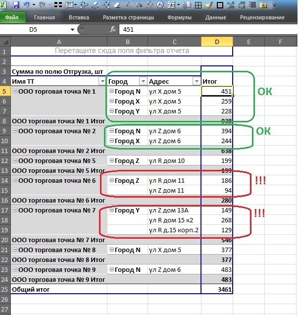
There are retail outlets detailed up to the lines of consignment notes, while it is allowed for points with the same name to have different addresses only if they are located in different cities, but there are points in the source dataset that have different addresses in the same city despite the fact that the names of the points are the same (the name of the outlet is unique, that is, it is a network unit or a stand-alone point). As a special case in aggregated form:
The following circumstances prevent the search and data cleansing by regular office resources:
• Data drill down to invoice lines
• Number of entries in several million lines
• Absence of sql toolkit (For example: Access - not included)
Of course, you can upload any free DBMS (even the desktop version, even the server version), but for this, you first need admin rights, and secondly, the article would no longer be about Power Pivot.
Task : for each atomic record, an additional calculated field is required, which will calculate for each name of the outlet a unique number of addresses within the same city. This field is required to quickly find all the names of outlets in the city, where the addresses are greater than 1.
I think it is most convenient to solve and tell iteratively, assuming that we have knowledge of DAX in the embryonic level.
Therefore, I propose for the time being to break away from the task and consider some basic aspects.
Step 1. How does a calculated column differ from a calculated measure?
Here is an example of a calculated column for extracting VAT from the shipping field with VAT using the built-in DAX formulas:
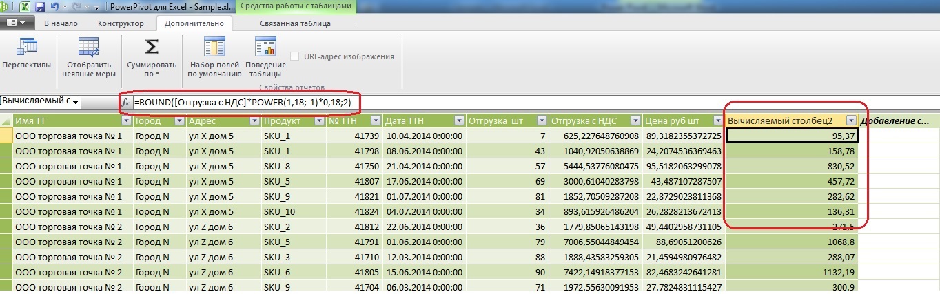
As you can see from the example, the calculated column (Let's call it VAT) works with each atomic entry horizontally.
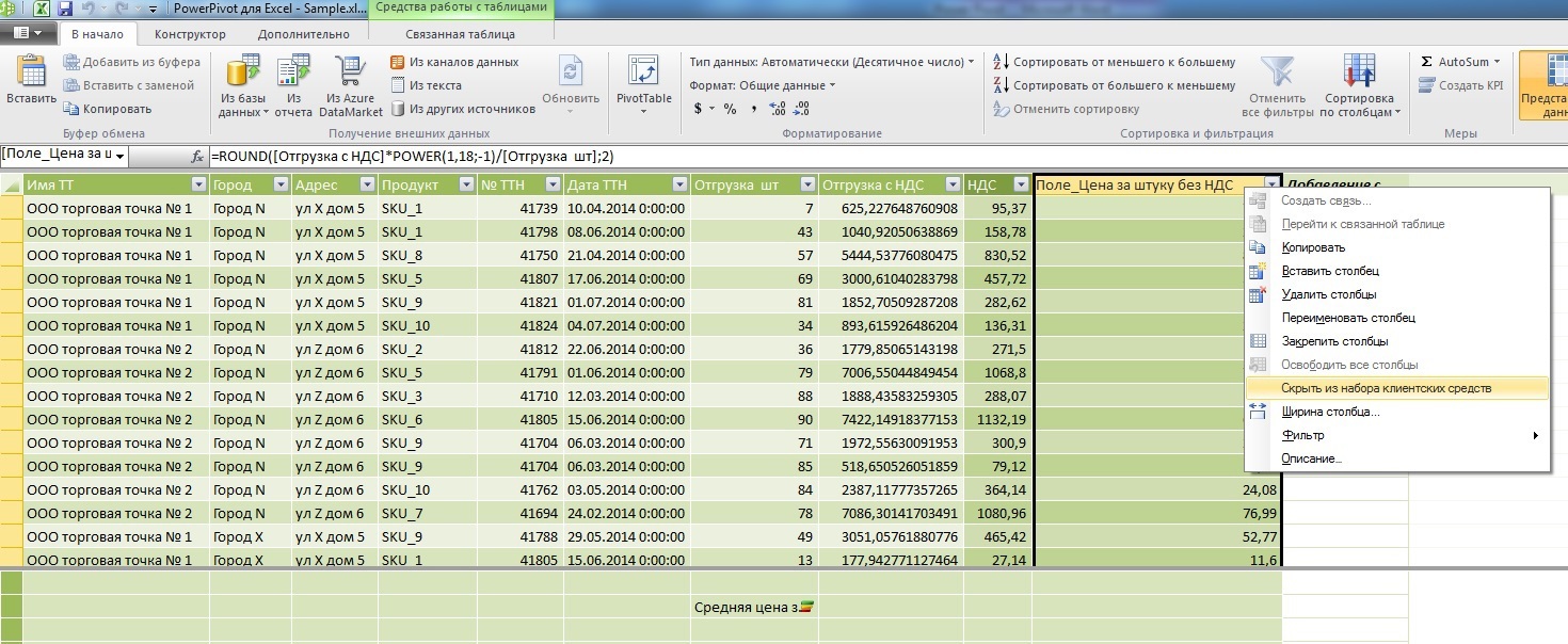
Now add a calculated field for the unit price excluding VAT:

Now, for comparison, let's add to the measure the calculation of the average price per item:
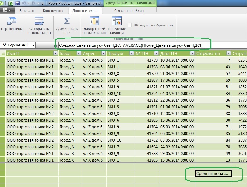
As can be seen from the formula, a measure works with a column of source data vertically, so it must always contain some function that works with a set (Sum, Average, Variance, etc.)
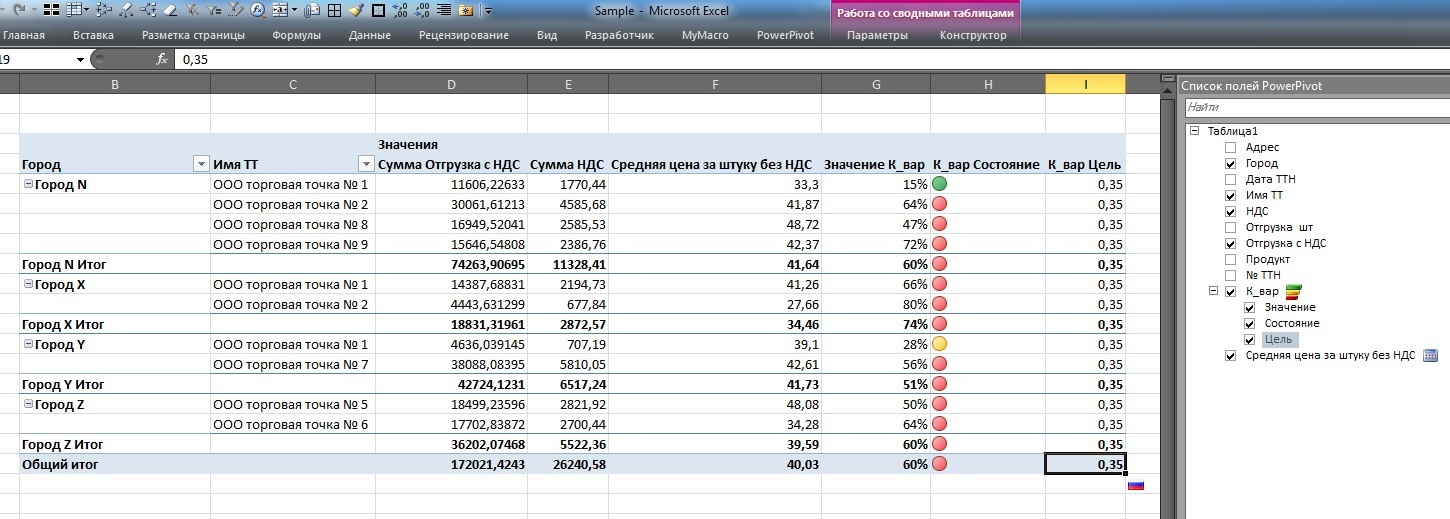
When returned to the Excel spreadsheet, it looks like this:
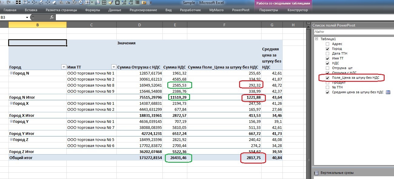
Note that if the calculated VAT field at each data level (green stroke at the point of sale, city, or total in the table) shows the amount that is correct in principle, the sum of the prices of the calculated price per item excluding VAT (red stroke) raises questions.
But the calculated measure "Average price per piece excluding VAT" is fully entitled to life within the framework of this analytical cube.
From here we conclude that the calculated field “Price per item without VAT” is an auxiliary tool for calculating the measure “Average price per item without VAT” and in order not to embarrass the user with this field, we will hide it from the list of client funds, leaving the average price measure.
Another difference to the measure from the column is that it allows you to add a visualization:
For example, we will build KPIs of price dispersion with a target border of 35% by dividing the root from the variance by the arithmetic average.

As a result, we see such a table in Excel (by the way, the calculated auxiliary price field is no longer in the list of available fields on the right):
A double click on the 80% ratio shows that prices really sausage around the average:

Stronger than with a ratio of 15%:

So, in this step, we looked at the main differences between the measures and the fields within PowerPivot.
Step 2. Complicate: Calculate the share of each record in total sales.
Here is the first example of comparing the approaches of the MS SQL Server and DAX window functions:
It is clear that within the framework of pivot tables this is done literally in 2 clicks with the mouse without touching the keyboard, but for understanding we will try this directly in PowerPivot using formulas.
On sql, I would write it this way (do not kick for flaws, because SQL Server does not check the syntax of Word):
Here, as you can see, the window opens through all dataset records, try a similar thing in PowerPivot:
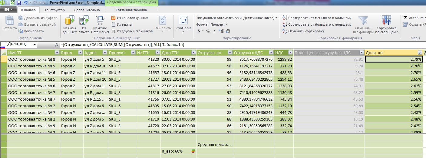
The main attention is drawn to the denominator: I have already mentioned above that the main difference between a calculated field and a measure is that in the formula field they count horizontally (within one record) and measures - vertically (within one attribute). Here we were able to cross field properties and measure property through the CALCULATE method. And if the width of the window in SQL, we adjusted through Over (), then here we did it through All ().
Let us now try, with this skill, to do something useful with our data, for example, remembering that the indicator of price dispersion around averages varied in a wide range, we will try to isolate statistical price emissions through the 3-sigma rule.
Window functions on sql will look like this:
But the same thing in the DAX:
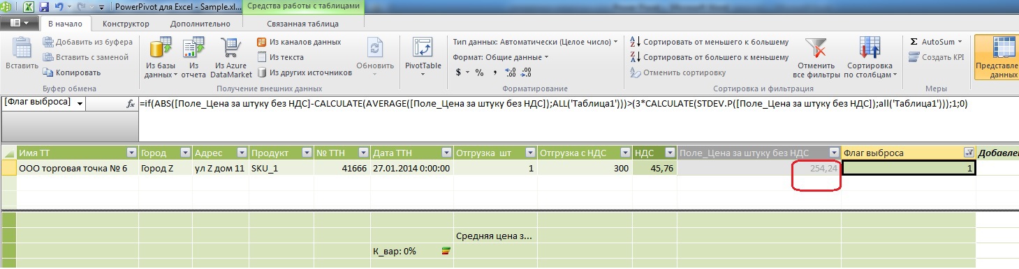
As you can see, the price is somewhat high with an arithmetic average of 40.03 rubles.
Step 3. We narrow the window.
Let us now try to count in the calculated field of each record the total number of records in the framework of the city to which this record belongs.
On MS sql Server window functions will look like this:
At DAX:
Pay attention to the difference in the display of data in the table, I specifically threw addresses into the area of measures to calculate their number and compare it with the new field that I entered in the header of the lines after the outlet.
The difference is clearly visible: if the usual calculation of the number of addresses goes for each point in the city and then only outputs the subtotal for the City aggregate, then using window functions allows you to assign the value of any aggregate to each atomic record, or use it in some intermediate calculations of the calculated field (as shown above).
Returning to the original problem
So, let me remind you, the initial formulation of the problem: for each atomic record, an additional calculated field is required, which counts for each name of the outlet a unique number of addresses within the same city. We do not forget that we have datasets detailed to the invoice lines, so before counting the addresses inside the window, they must be grouped.
SQL Server Query:
Now nothing prevents us from doing this in DAX:
As a result, we had the opportunity to select suspicious records, where there is more than 1 address to the same point in the same city.

Of course, in the process of learning (having run through the look at other formulas) it becomes clear that DAX in PowerPivot is much more powerful than shown in this topic, but embracing the immense at a time will definitely not work.
I hope it was interesting.
Read the article here.
While working in the field of analytics and monitoring various BI tools, sooner or later you come across a review or mention of the Power Pivot Excel add-in. In my case, an acquaintance with him happened at the Microsoft Data Day conference.
After the presentation, the tool did not leave much of an impression: Yes, it is free (under the Office license), yes - there is some ETL functionality in terms of receiving data from disparate sources (DB, csv, xls, etc.), Join these sources and feeding records into the operating system by orders of magnitude above 1 million rows in Excel. In short, looked and forgot.
')
And I had to remember when it became necessary to identify certain phenomena in the data
This article was inspired by the fact that there is not a lot of any detailed information about specific methods of work in Runet, more and more about the stars, so I decided to write this review while studying this tool.
Actually, the statement of the problem (by an impersonal example) is as follows:
In the csv file source data:
There are retail outlets detailed up to the lines of consignment notes, while it is allowed for points with the same name to have different addresses only if they are located in different cities, but there are points in the source dataset that have different addresses in the same city despite the fact that the names of the points are the same (the name of the outlet is unique, that is, it is a network unit or a stand-alone point). As a special case in aggregated form:
The following circumstances prevent the search and data cleansing by regular office resources:
• Data drill down to invoice lines
• Number of entries in several million lines
• Absence of sql toolkit (For example: Access - not included)
Of course, you can upload any free DBMS (even the desktop version, even the server version), but for this, you first need admin rights, and secondly, the article would no longer be about Power Pivot.
Task : for each atomic record, an additional calculated field is required, which will calculate for each name of the outlet a unique number of addresses within the same city. This field is required to quickly find all the names of outlets in the city, where the addresses are greater than 1.
I think it is most convenient to solve and tell iteratively, assuming that we have knowledge of DAX in the embryonic level.
Therefore, I propose for the time being to break away from the task and consider some basic aspects.
Step 1. How does a calculated column differ from a calculated measure?
Here is an example of a calculated column for extracting VAT from the shipping field with VAT using the built-in DAX formulas:
=ROUND([ ]*POWER(1,18;-1)*0,18;2)As you can see from the example, the calculated column (Let's call it VAT) works with each atomic entry horizontally.
Now add a calculated field for the unit price excluding VAT:
=ROUND([ ]*POWER(1,18;-1)/[ ];2)Now, for comparison, let's add to the measure the calculation of the average price per item:
: =ROUND(AVERAGE([_ ]);2)As can be seen from the formula, a measure works with a column of source data vertically, so it must always contain some function that works with a set (Sum, Average, Variance, etc.)
When returned to the Excel spreadsheet, it looks like this:
Note that if the calculated VAT field at each data level (green stroke at the point of sale, city, or total in the table) shows the amount that is correct in principle, the sum of the prices of the calculated price per item excluding VAT (red stroke) raises questions.
But the calculated measure "Average price per piece excluding VAT" is fully entitled to life within the framework of this analytical cube.
From here we conclude that the calculated field “Price per item without VAT” is an auxiliary tool for calculating the measure “Average price per item without VAT” and in order not to embarrass the user with this field, we will hide it from the list of client funds, leaving the average price measure.
Another difference to the measure from the column is that it allows you to add a visualization:
For example, we will build KPIs of price dispersion with a target border of 35% by dividing the root from the variance by the arithmetic average.
_:=STDEV.P([_ ])/AVERAGE([_ ])As a result, we see such a table in Excel (by the way, the calculated auxiliary price field is no longer in the list of available fields on the right):
A double click on the 80% ratio shows that prices really sausage around the average:
Stronger than with a ratio of 15%:
So, in this step, we looked at the main differences between the measures and the fields within PowerPivot.
Step 2. Complicate: Calculate the share of each record in total sales.
Here is the first example of comparing the approaches of the MS SQL Server and DAX window functions:
It is clear that within the framework of pivot tables this is done literally in 2 clicks with the mouse without touching the keyboard, but for understanding we will try this directly in PowerPivot using formulas.
On sql, I would write it this way (do not kick for flaws, because SQL Server does not check the syntax of Word):
Begin Select 't1. ', 't1.', 't1.', 't1.', 't1.№ ', 't1. ', 't1., ', 't1. ', 't1., '/sum('t1., ') over () as share from Table as t1 order by 't1., '/sum('t1., ') desc Here, as you can see, the window opens through all dataset records, try a similar thing in PowerPivot:
=[ ]/CALCULATE(SUM([ ]);ALL('1'))The main attention is drawn to the denominator: I have already mentioned above that the main difference between a calculated field and a measure is that in the formula field they count horizontally (within one record) and measures - vertically (within one attribute). Here we were able to cross field properties and measure property through the CALCULATE method. And if the width of the window in SQL, we adjusted through Over (), then here we did it through All ().
Let us now try, with this skill, to do something useful with our data, for example, remembering that the indicator of price dispersion around averages varied in a wide range, we will try to isolate statistical price emissions through the 3-sigma rule.
Window functions on sql will look like this:
Select 't1. ', 't1.', 't1.', 't1.', 't1.№ ', 't1. ', 't1., ', 't1. ', 't1. ', CASE WHEN ABS('t1. ' - AVG('t1. ') OVER() ) > 3 * STDEV('t1. ') OVER() THEN 1 ELSE 0 END as Outlier from Table as t1 Go But the same thing in the DAX:
=if(ABS([_ ]-CALCULATE(AVERAGE([_ ]);ALL('1')))>(3*CALCULATE(STDEV.P([_ ]);all('1')));1;0)As you can see, the price is somewhat high with an arithmetic average of 40.03 rubles.
Step 3. We narrow the window.
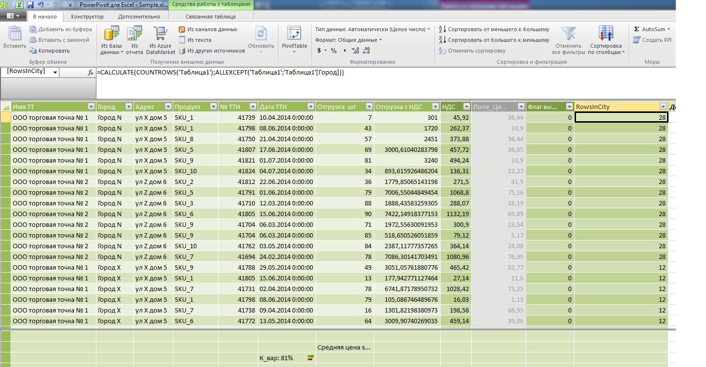
Let us now try to count in the calculated field of each record the total number of records in the framework of the city to which this record belongs.
On MS sql Server window functions will look like this:
Select 't1. ', 't1.', 't1.', 't1.', 't1.№ ', 't1. ', 't1., ', 't1. ', 't1. ', count('t1.*) OVER( partition by 't1.' ) as cnt from Table as t1 Go At DAX:
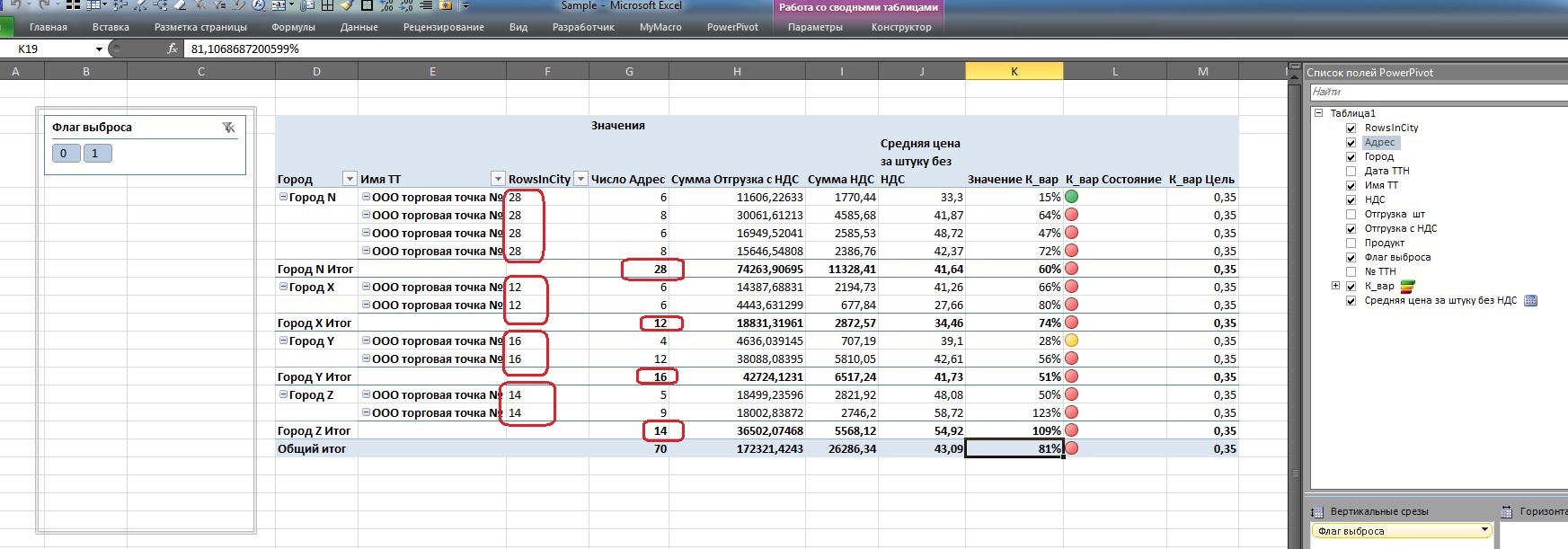
=CALCULATE(COUNTROWS('1');ALLEXCEPT('1';'1'[]))Pay attention to the difference in the display of data in the table, I specifically threw addresses into the area of measures to calculate their number and compare it with the new field that I entered in the header of the lines after the outlet.
The difference is clearly visible: if the usual calculation of the number of addresses goes for each point in the city and then only outputs the subtotal for the City aggregate, then using window functions allows you to assign the value of any aggregate to each atomic record, or use it in some intermediate calculations of the calculated field (as shown above).
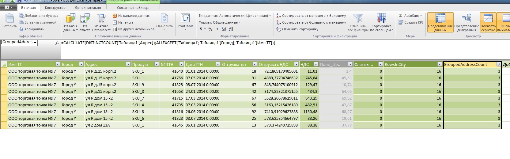
Returning to the original problem
So, let me remind you, the initial formulation of the problem: for each atomic record, an additional calculated field is required, which counts for each name of the outlet a unique number of addresses within the same city. We do not forget that we have datasets detailed to the invoice lines, so before counting the addresses inside the window, they must be grouped.
SQL Server Query:
With a1 as (Select 't1. ', 't1.', 't1.', 't1.', 't1.№ ', 't1. ', 't1., ', 't1. ', 't1. ', count(Distinct 't1.') OVER( partition by 't1.', 't1. ' ) as adrcnt from Table as t1) Select * from a1 where adrcnt>1 Now nothing prevents us from doing this in DAX:
=CALCULATE(DISTINCTCOUNT('1'[]);ALLEXCEPT('1';'1'[];'1'[ ]))As a result, we had the opportunity to select suspicious records, where there is more than 1 address to the same point in the same city.
Of course, in the process of learning (having run through the look at other formulas) it becomes clear that DAX in PowerPivot is much more powerful than shown in this topic, but embracing the immense at a time will definitely not work.
I hope it was interesting.
Read the article here.
Source: https://habr.com/ru/post/245631/
All Articles