Quickhull algorithm for finding a convex hull
As the definition says, the convex hull of some set  - this is the smallest convex set
  containing many . The convex hull of a finite set of pairwise distinct points is a polyhedron.
To implement the one-dimensional case of the Quickhull algorithm, the std :: minmax_element function is appropriate . In the network you can find many implementations of the Quickhull algorithm for a flat case. However, for the case of an arbitrary dimension, only one heavyweight implementation from qhull.org is immediately available .
In brackets next to the terms, I will give a translation into English (in the style of Tu'bo, sorry). This can be useful for those who are not familiar with the terms and will read the English texts on the links, or decide to deal with the texts of the source code.
The “canonical” implementation mentioned above is written in C (there is C ++ binding), it has been used for a long time and widely (as part of the GNU Octave and MATLAB packages) and, therefore, is well tested. But if you decide to isolate code that relates only to one Quickhull algorithm, you will encounter difficulties. For the simplest applications, I would like to be able to get by with something more compact. Having a little tried, I wrote my own implementation ( https://github.com/tomilov/quickhull ): this is the only class, without dependencies. About 750 lines in total.
Starting to work with multidimensional entities, you understand that some analogies with the usual two-dimensional and three-dimensional objects are valid. It is necessary to streamline knowledge: introduce some new terms and clarify the relationship between them.
For a programmer, geometric objects are primarily data structures. To begin with, I will give geometric definitions (not very strict). Further in the text will be given descriptions of the corresponding data structures, convenient to store data and operate with them quite effectively.
Denote the dimension of the space as .
.
The face of a polyhedron, its boundaries, the boundaries of its boundaries, etc. in English are called face. Dame link to a good resource, where it is logically justified that in dimensional space visible or observable objects may be only  -dimensional objects, i.e. boundaries -dimensional objects. The English term facet is precisely the observed face. Straight (born straight line) - is always a one-dimensional entity. The point (vertex) can be considered zero-dimensional in this gradation.
Dealing with some set of points, we can proceed to the consideration of the corresponding set of
  vectors by subtracting one of the points from all the others. Thus, we will, as it were, designate this point as the origin of coordinates. If all points lie in the same plane, then the plane is displaced in such a way that it begins to pass through the origin. Affinity independence points is performed when linear independence is performed th corresponding vector. The definition of linear independence of vectors is probably already familiar to you. So in -dimensional space can not choose more
  points so that they are all affinely independent. Let me explain this: in a three-dimensional space, a triangle (the face of a three-dimensional simplex - a tetrahedron) is defined by three points (not lying on one straight line, of course); a single plane passes through these three points; any point of this plane added to the set of three vertices of the triangle will transform a set of three affinely independent points into a set of 4 affinely dependent ones. The analogy is valid for other dimensions.
Among other things, it is necessary to introduce the concept of hypervolume (eng. Hypervolume).
')
The Quickhull algorithm itself for the case of arbitrary dimension was proposed in Barber, C. Bradford; Dobkin, David P .; Huhdanpaa, Hannu (1 December 1996). "The quickhull algorithm for convex hulls". ACM Transactions on Mathematical Software 22 (4): 469–483 . The “canonical” implementation in C from the authors is located on the already mentioned site http://qhull.org/ , the repository with the C ++ interface https://gitorious.org/qhull/qhull . I will quote the algorithm from the original source:
A convex hull is a list of faces.
As you can see, we need to start with some starting simplex . To do this, you can choose any affine independent points, but it is better to use some cheap heuristics. The main requirement at this step is that our simplex should not be “narrow” if possible (eng. Narrow). This is important if you use floating-point arithmetic (eng. Floating-point arithmetic). In the original implementation, points with maximum and minimum values of coordinates are used (obviously, they will also be included in the set of vertices of the convex hull). Starting from the starting simplex, at each subsequent step we will get more and more polyhedra, the constant property of which will always be its convexity. I will call it a temporary polyhedron .
Next, we must distribute the remaining points to the so-called lists of external points (outside sets) of the faces - these are lists of points that are maintained for each face and which are still not considered (hereinafter - unassigned, English unassigned) points that are relatively face planes on the other side than the interior of the simplex (or a temporary polyhedron in the future). Here we use the property of a convex polyhedron (and simplex in particular) that it lies entirely in only one of the two half-spaces obtained by splitting the whole space with the plane of each face. From this property follows the fact that if a point does not fall into any of the lists of external points of the faces of the convex hull, then it is reliably located inside it. In the future, the algorithm will need information about which of the points contained in the list of external points and the most distant from the plane of the face, therefore, adding points to the list of external points, you need to save information about which one is the furthest. Any point falls only in one list of external points. The asymptotic complexity is not affected by how exactly the points are distributed among the lists.
At this stage, I need to digress and tell how to set the face, how to calculate the distance to it, how to determine the orientation of a point relative to the face.
Now we are able to describe the face plane, but there is one ambiguity: how to choose the order of listing points in the lists of vertices of faces of the starting simplex? Authors do not keep the list of vertices ordered. They act differently. By setting the plane equation for an arbitrary but fixed order of the vertices, they find out the orientation of an internal point relative to this plane. That is, the oriented distance is calculated. If the distance is negative, they change the sign of the coordinates of the normal to the hyperplane and its offset from the origin. Or set the value of the flag, indicating that the face is inverted (English flipped). The internal point for a convex polyhedron will be the arithmetic average of at leastits vertices (the so-called center of mass, if we take all the vertices).
For each face, in addition to specifying a list of vertices, a list of external points, you must specify a list of adjacent (eng. Adjacency list) faces. For each face it will contain exactly items.Since the starting simplex contains a face, it is obvious that for any of its faces, all other faces ( pieces) will fall into the list of adjacent faces .
Now there is a temporary polygon with which you can work in the main loop. In the main cycle, this temporary polygon is completed by “capturing” more and more space, and with it the points of the original set, until a moment comes when there will not be a single point outside the polyhedron. Further I will describe this process in more detail. Namely, the way it works in my implementation.
The main loop is a loop along edges. At each iteration, among the faces with non-empty lists of external points, the best face is selected (eng. Best facet); best in the sense that the farthest point from the list of external points is farther from the face than other faces. The cycle ends when there are no faces with non-empty lists of external points.
In the body of the main loop, the selected face is deleted as a convex hull that is not the face of a convex hull. But beforehand, she "understands the components." From the list of external points, the farthest point is extracted (eng. Furthest point) - it is probably the top of the convex hull. The remaining points are moved to a separate temporary list of unassigned points.
 .Further, according to the lists of adjacent faces, starting from the list of faces , the adjacency graph of the faces of the temporary polyhedron is bypassed and each face is added to the list of already visited (eng. Visited) faces and tested for visibility (eng. Visibility) from a point .If the face is invisible from a point , then its adjacent faces will not be further circumvented, otherwise they are bypassed. If the next visible face among neighboring faces has invisible ones from a point , then it falls into the list of border visible faces (the English before-the-horizon, as opposed to over-the-horizon, is “over the horizon”). But if all adjacent faces are visible, then such a face is added to the list of faces to be deleted. After traversing the adjacency graph of faces, the list of boundary visible faces and the list of faces to be deleted all contain all visible from the point.facets. Now all faces are deleted from the list for deletion. Moreover, each deleted face is not removed from the lists of neighboring faces from its neighbors. It is safe to do so, because even if the neighboring face is the visible edge of the border, from the list of its neighboring faces only information about the proximity to the invisible from the point is used in the future . Following the list of faces to be deleted is a list of visible edges. Each boundary visible edge is “parsed” (then we will need its list of adjacent faces and a list of vertices) and is deleted. For each boundary visible face, new faces are created (from one topieces), which are added to the list of new faces. At the same time, a list of its neighboring faces is viewed, and for each face from this list, which is invisible, a common edge with a given visible boundary is searched for. The vertices common to the invisible and boundary visible edges (that is, the vertices of the common edge) are written out to the list of vertices of a new face, moreover in the order in which they are written in the list of vertices of the boundary visible face. The edge (eng. Horizon ridge), by the way, is part of the horizon of that part of the surface of the temporary polyhedron that is visible from the point . The only vertex of the visible boundary that does not belong to this edge is replaced by the point in the list of vertices of the new face, the rest of the vertices are the same as in the (ordered) list of vertices of the boundary visible face and stand in the same places. Thus, the constructed list of vertices of the new facet guarantees its correct orientation, that is, when calculating its normalized plane equation, the normal will be directed outside the time polyhedron and the offset value will receive the correct sign. After all the boundary visible edges are processed, we have a list of new faces. The hyperplane equations for these faces can be calculated immediately after we have vertex lists for them. Also, when creating new faces, one can add one facet to their lists of adjacent faces, namely, the corresponding invisible face that was adjacent to the boundary visible face when forming the list of vertices of a new face. Obviously the restNeighboring faces must be searched for among other new faces.
As it turned out (when sampling by the profiler from Google Performance Tools ), the most time in the case of large dimensions and / or poor input data (that is, when most of the points are vertices of a convex hull) the algorithm spends searching for neighboring faces for new faces. In my implementation, the algorithm was initially very simple: all possible pairs (two nested loops) of faces from the list of new faces were searched and comparisons were made (by the number from the input list of points) of vertex lists with one mismatch (modified algorithm std :: set_difference or std :: set_symmetric_difference ). I.e comparisons, where - the number of new faces. But later I managed to win a pair (binary =) orders in the speed of searching for neighboring ones using ordered associative arrays ( std :: set ) in this narrow place. In general, there is a whole area of knowledge that is associated with this task (identifying neighbors) - this is locality-sensitive hashing . In the original implementation of qhulljust hashes are used (not LSH). It contains a separate data structure for each edge (two faces) (a list of edge vertices and information about faces “above” and “below” an edge), each face contains a list of its edges. To determine the neighborhood of the faces (among the faces from the list of new faces) for all edges of the faces, an associative unordered array of hashes of arrays of their vertices is created (with one skip (English skip) and one dropped vertex ). I.e
  saves hashes. If there is a collision (and the subsequent complete coincidence of the lists) of hashes, then (obviously) these two faces have a common edge (the hash, by the way, can be removed to reduce the hash table) and each of them can be added to the list of adjacent faces of the other. I do not use this method, since neither in the standard library nor in the STL there is such a tool as hash combiner (upd. Received information that the best choice is just XOR). I didn’t want to specialize without the information-theoretical justification of the correctness of std :: hash for std :: vector <std :: size_t> . That is why I used associative orderededge container for finding adjacent faces. As a result (apparently) my implementation of the algorithm loses qhull in speed asymptotically in from
 before
  times (for all sorts of input data).
The example is the “canonical” implementation of the Quickhull qhull algorithm, installed through the package manager (in Ubuntu 14.04 LTS). To generate input from the same qhull-bin package, the rbox utility was used . The rbox tn D4 30000 s> /tmp/qhuckhull.txt command creates a file with coordinates of 30,000 points on a four-dimensional sphere. The rbox tn D10 30 s> /tmp/quickhull.txt command creates a file with the coordinates of 30 points on a ten-dimensional sphere. The amount of memory that the program spends can be seen in the output of the / usr / bin / time utility with the -v option . Thus, in the output / usr / bin / time -v bin / quickhull /tmp/quickhull.txt | head -7 you can find out the consumption of both memory and processor time (cleared from the time to read files and output to the terminal) for my implementation, and in the output / usr / bin / time -v qconvex s Qt Tv TI /tmp/quickhull.txt - for the “canonical” implementation of qhull .
I determine the correctness of my implementation by the coincidence of the number of faces of the convex hulls. But for debugging (in two-dimensional and three-dimensional modes) at some stage I implemented step-by-step (via the pause command) animated output in gnuplot format. Somewhere in commits it is. The output of the program is a convex hull and a numbered set of input points represented in the gnuplot format.
In addition, somehow I started writing (but did not finish) the randombox utility, an analogue of rbox . randombox was conceived as a utility that generates points uniformly distributed in space (English uniform spatial distribution), in contrast to rbox , which generates points that are not evenly distributed. randombox can generate sets of points bounded by a simplex (of any dimension that can be embedded in space with points), on a unit sphere (in the unit sphere), in a ball (English ball), on the surface of a single “diamond-shaped” polyhedron (Eng. unit diamond), inside a unit cube (English unit cube), inside a parallelotope, within the standard unit simplex (English unit simplex), and also projects a set of points into the volume of the cone (English cone) or cylinder (English cylinder ). To generate coordinates that are evenly distributed within an arbitrary speclex (embedded in space), I found a numerically stable algorithm on the Internet (through the Dirichlet distribution), and also came up with my own algorithm, which does not have this property. In the end, chose the first.
In order to “feel” the bulging shells with a glance using gnuplot , from the project root enter the command rbox n D3 40 t | bin / quickhull> /tmp/quickhull.plt && gnuplot -p -e "load '/tmp/quickhull.plt'" . rbox n D3 40 t will generate 40 points inside the bounding cube (eng. bounding box). The key t specifies the use of the current time (in seconds) as the initial PRNG value. To get points on a sphere, you need to add the key s . It is also interesting to see how nonsimplicial faces are broken: rbox n D3 c - cube, rbox n D3 729 M1,0,1 -
  points located in whole nodes. The convex shell of the helix looks beautiful (eng. Helix): rbox n D3 50 l . In the case of the simultaneous location of a large number of points coplanar to the edges, the constant eps begins to play a great role for the correctness of the results, which is set when constructing the algorithm object. For example, if you use std :: numeric_limits <value_type> :: epsilon () as a small value, then in the case of a “rotated” cube of 64 integer points of rbox n D3 64 M3.4, as a result of the algorithm, an incorrect which is a convex polygon.
The result of my work was the release of the Quickhull algorithm in C ++, quite compact and not very slower than the implementation with qhull.org . The algorithm receives at the input the value of the dimension of space, the value of the small constant eps and the set of points represented as a range defined by a pair of iterators, as is customary in STL. At the first stage of create_simplex, the starting simplex is built and the point basis of the affine (sub) space containing the input points is returned. If the number of points in the basis is greater than the dimension of the Euclidean space containing the points, then the algorithm for completing the construction of the convex hull must be run. At the output, the algorithm will give an array of data structures describing the faces of the convex hull of the input set, which is the answer. In case of failure, we have a point basis of some subspace of lower dimension, which contains all points. Using the Householder algorithm, you can in some way rotate the input set, while vanishing the highest coordinates of the points. Such coordinates can be discarded and the Quickhull algorithm can be applied already in a space of lower dimension.
This algorithm has many applications. In addition to finding the convex hull as such, due to the fact that there is a connection between the convex hull , the Delaunay triangulation and the Voronoi diagram , it is easy to find applications of the algorithm "indirectly".
This implementation has already come in handy for some people , and was paid for with gratitude (in Acknowledgments), which is very nice.
06/24/2015: A check of the convexity of the resulting geometric structure was added according to the algorithm of Kurt Mehlhorn, Stefan Näher, Thomas Schilz, Stefan Schirra, Michael Seel, Raimund Seidel, and Christian Uhrig. Checking geometric programs or verification of geometric structures. In Proc. 12th Annu. ACM Sympos. Comput. Geom., Pages 159-165, 1996 .
06/24/2015: The faces of the resulting polyhedron now contain sets of vertices and indices of neighboring faces arranged in such a way that the face is the opposite one and the corresponding vertex. This makes the structure much more convenient to use in some cases.
06.24.2015 G .: Now for the determination of the neighborhood of newly obtained faces, their hashes are used.
- this is the smallest convex set containing many . The convex hull of a finite set of pairwise distinct points is a polyhedron.To implement the one-dimensional case of the Quickhull algorithm, the std :: minmax_element function is appropriate . In the network you can find many implementations of the Quickhull algorithm for a flat case. However, for the case of an arbitrary dimension, only one heavyweight implementation from qhull.org is immediately available .
In brackets next to the terms, I will give a translation into English (in the style of Tu'bo, sorry). This can be useful for those who are not familiar with the terms and will read the English texts on the links, or decide to deal with the texts of the source code.
The “canonical” implementation mentioned above is written in C (there is C ++ binding), it has been used for a long time and widely (as part of the GNU Octave and MATLAB packages) and, therefore, is well tested. But if you decide to isolate code that relates only to one Quickhull algorithm, you will encounter difficulties. For the simplest applications, I would like to be able to get by with something more compact. Having a little tried, I wrote my own implementation ( https://github.com/tomilov/quickhull ): this is the only class, without dependencies. About 750 lines in total.
Geometric concepts.
Starting to work with multidimensional entities, you understand that some analogies with the usual two-dimensional and three-dimensional objects are valid. It is necessary to streamline knowledge: introduce some new terms and clarify the relationship between them.
For a programmer, geometric objects are primarily data structures. To begin with, I will give geometric definitions (not very strict). Further in the text will be given descriptions of the corresponding data structures, convenient to store data and operate with them quite effectively.
Denote the dimension of the space as
.- Simplex (English simplex) is set affinely independent (English affinely independent) point. I will explain further affinity independence below. These points are called vertices (eng. Vertex, pl. Vertices).
- The polyhedron (syn. Polytopic, polyhedron, polyhedron, English polytope, polyhedron) is defined at least affinely independent point (vertex); simplex (English simplicial polytope) - the simplest case -dimensional body, polyhedra with a smaller number of vertices will necessarily have zero -dimensional volume.
- Parallelotope (English parallelotope) is a generalization of a flat parallelogram and a volume parallelepiped. For simplex you can build corresponding parallelotops (they will all have the same volume, equal to
 to the volumes of the simplex), taking as the generators (vectors) of the parallelotope the vectors that go from one fixed vertex to the others tops.
 - I will not give here the concept of a convex polyhedron (born convex polytope, convex polyhedron), your intuitive idea of it will fit. A simplex, as a special case of a polyhedron, is always convex.
- I will not give the concept of a plane either. Just note that it has one less dimension than the space into which it is embedded.
- Simplicial face (born simplicial facet) is defined affinely independent points (vertices). Further, we will speak only of simplicial objects (except for a convex polyhedron), so I will omit the definition of “simplicial”. Many of the assertions will continue to be valid only for non-degenerate (all points are pairwise different) cases of simplicial geometric objects.
- Edge (English ridge) is defined as the intersection of two faces and has the top. Two faces can have only one common edge. One facet, therefore, may have neighbors through ribs.
- Peak (eng. Peak) is determined
 points. Here, an intuitive analogy with three-dimensional space can float, since the concept of a peak and a vertex do not coincide, but we will not operate with such objects. A face can have any number of neighboring faces through the peak, hence we can conclude that storing the graph of adjacency of faces through peaks is expensive and in memory and at the cost of maintaining the relevance of the data structures during any transformations.
The face of a polyhedron, its boundaries, the boundaries of its boundaries, etc. in English are called face. Dame link to a good resource, where it is logically justified that in
dimensional space visible or observable objects may be only -dimensional objects, i.e. boundaries -dimensional objects. The English term facet is precisely the observed face. Straight (born straight line) - is always a one-dimensional entity. The point (vertex) can be considered zero-dimensional in this gradation.Dealing with some set of
points, we can proceed to the consideration of the corresponding set of vectors by subtracting one of the points from all the others. Thus, we will, as it were, designate this point as the origin of coordinates. If all points lie in the same plane, then the plane is displaced in such a way that it begins to pass through the origin. Affinity independence points is performed when linear independence is performed th corresponding vector. The definition of linear independence of vectors is probably already familiar to you. So in -dimensional space can not choose more points so that they are all affinely independent. Let me explain this: in a three-dimensional space, a triangle (the face of a three-dimensional simplex - a tetrahedron) is defined by three points (not lying on one straight line, of course); a single plane passes through these three points; any point of this plane added to the set of three vertices of the triangle will transform a set of three affinely independent points into a set of 4 affinely dependent ones. The analogy is valid for other dimensions.Among other things, it is necessary to introduce the concept of hypervolume (eng. Hypervolume).
')
Hyper volume
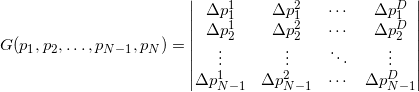
Any considered object from the series simplex , edge , edge , peak , etc. bounded in the corresponding subspace. The “amount of space” that such an object occupies can be measured / determined / defined. For a one-dimensional direct measure is called length; for a two-dimensional plane, the measure is called area; for a three-dimensional body - volume. The concept can be generalized by naming it a D-dimensional volume or a D-hyper volume. For a simplex formed by pairwise different points  (the order of the enumeration of points is important), you can calculate the hyper volume as follows :


Here we wrote out the coordinates of the vectors in the line. Similar formulas and reasoning can be given for column vectors (that is, if we transpose all matrices, then this will not affect the result and conclusions).
The divisor of the determinant in the formula above is the number of simplices (they all have the same volume) into which the parallelotope can be broken. built on vectors
  . Accordingly, the determinant itself is a volume of a parallelotope. For those interested in the bases underlying this statement, I recommend reading about the determinant of the Gram matrix and its geometric interpretation.
It should be noted that this measure will have a nonzero value for “volume” objects, and it can also be both positive and negative. It is easy to understand the meaning of the sign from the following considerations: when exchanging the two points of the simplex, we get the sign change of the determinant; the order of points is the “left- and right orientation” of the simplex. On a plane, it's easy to imagine: if the sides of a triangle listed counterclockwise
  , then the determinant is positive
  otherwise
  - negative
  . For a tetrahedron, the sign will depend on the order in which (clockwise or counterclockwise) the first 3 points will be listed when looking at them from the last. Thus, in the future, when specifying geometric objects, we must accept that the order of enumeration of points must be fixed.
We can omit the factor before the determinant, since the algorithm will use only information about the sign of the magnitude of the oriented hypervolume.
The determinant is zero if at least two lines are linearly dependent (remember that the points are pairwise different, that is, not one line is non-zero). It is easy to verify the consistency of the above arguments about affine-dependent points and linearly dependent vectors corresponding to them.
The absolute value of the determinant will not be affected by exactly which point is subtracted during the transition to the vectors - only the sign. It is always necessary to subtract the last point from the first one, otherwise for similarly oriented similar objects used in the future, the sign of the measure will be different in even and odd dimensions.
What to do with the measure for objects nested in a space of too large dimension, for example, with edges? If we construct the matrix in the same way as shown above, it will be rectangular. Determinant from such a matrix will not work. It turns out that the formula can be generalized (this generalization is related to the Binet-Cauchy formula ) using the same matrix made up of row vectors:


For affinely independent pairwise distinct points, the matrix under the determinant always turns out to be square positive-definite, while the determinant of such a matrix is always a positive number. For affine dependent points, the matrix will be singular (that is, its determinant is zero). It is clear that the measure is always non-negative and we have no information about orientation.
On the one hand, the determinant of the product of square matrices is equal to the product of determinants, on the other hand, the determinant of the transposed square matrix coincides with the determinant of the original matrix, so the last formula reduces to the formula for the points, except for the root of the square, i.e. module, which we can omit, in order to obtain additional information about the relative orientation of points in space.
(the order of the enumeration of points is important), you can calculate the hyper volume as follows :Here we wrote out the coordinates of the vectors in the line. Similar formulas and reasoning can be given for column vectors (that is, if we transpose all matrices, then this will not affect the result and conclusions).
The divisor of the determinant in the formula above is the number of simplices (they all have the same volume) into which the parallelotope can be broken.
built on vectors . Accordingly, the determinant itself is a volume of a parallelotope. For those interested in the bases underlying this statement, I recommend reading about the determinant of the Gram matrix and its geometric interpretation.It should be noted that this measure will have a nonzero value for “volume” objects, and it can also be both positive and negative. It is easy to understand the meaning of the sign from the following considerations: when exchanging the two points of the simplex, we get the sign change of the determinant; the order of points is the “left- and right orientation” of the simplex. On a plane, it's easy to imagine: if the sides of a triangle
listed counterclockwise , then the determinant is positive otherwise - negative . For a tetrahedron, the sign will depend on the order in which (clockwise or counterclockwise) the first 3 points will be listed when looking at them from the last. Thus, in the future, when specifying geometric objects, we must accept that the order of enumeration of points must be fixed.We can omit the factor before the determinant, since the algorithm will use only information about the sign of the magnitude of the oriented hypervolume.
The determinant is zero if at least two lines are linearly dependent (remember that the points are pairwise different, that is, not one line is non-zero). It is easy to verify the consistency of the above arguments about affine-dependent points and linearly dependent vectors corresponding to them.
The absolute value of the determinant will not be affected by exactly which point is subtracted during the transition to the vectors - only the sign. It is always necessary to subtract the last point from the first one, otherwise for similarly oriented similar objects used in the future, the sign of the measure will be different in even and odd dimensions.
What to do with the measure for objects nested in a space of too large dimension, for example, with edges? If we construct the matrix in the same way as shown above, it will be rectangular. Determinant from such a matrix will not work. It turns out that the formula can be generalized (this generalization is related to the Binet-Cauchy formula ) using the same matrix made up of row vectors:
For affinely independent pairwise distinct points, the matrix under the determinant always turns out to be square positive-definite, while the determinant of such a matrix is always a positive number. For affine dependent points, the matrix will be singular (that is, its determinant is zero). It is clear that the measure is always non-negative and we have no information about orientation.
On the one hand, the determinant of the product of square matrices is equal to the product of determinants, on the other hand, the determinant of the transposed square matrix coincides with the determinant of the original matrix, so the last formula reduces to the formula for
the points, except for the root of the square, i.e. module, which we can omit, in order to obtain additional information about the relative orientation of points in space.Algorithm.
The Quickhull algorithm itself for the case of arbitrary dimension was proposed in Barber, C. Bradford; Dobkin, David P .; Huhdanpaa, Hannu (1 December 1996). "The quickhull algorithm for convex hulls". ACM Transactions on Mathematical Software 22 (4): 469–483 . The “canonical” implementation in C from the authors is located on the already mentioned site http://qhull.org/ , the repository with the C ++ interface https://gitorious.org/qhull/qhull . I will quote the algorithm from the original source:
 create a simplex of d + 1 points
 for each facet F
	 for each unassigned point p
		 if p is above F
			 assign p to f`s outside set
 for each facet with a non-empty outside set
	 select the furthest point of f set
	 initialize the visible set V to F
	 for all unvisited neighbors n of facets in v
		 if p is above N
			 add N to V
	 the set of horizon ridge
	 for each ridge R in H
		 create a new facet from R and P
		 link the new facet to its neighbors
	 for each new facet F '
		 set of face to face
			 if q is above F '
				 assign q to F'`s outside set
	 delete the facets in v
A convex hull is a list of faces.
Starting simplex.
As you can see, we need to start with some starting simplex . To do this, you can choose any
affine independent points, but it is better to use some cheap heuristics. The main requirement at this step is that our simplex should not be “narrow” if possible (eng. Narrow). This is important if you use floating-point arithmetic (eng. Floating-point arithmetic). In the original implementation, points with maximum and minimum values of coordinates are used (obviously, they will also be included in the set of vertices of the convex hull). Starting from the starting simplex, at each subsequent step we will get more and more polyhedra, the constant property of which will always be its convexity. I will call it a temporary polyhedron .Heuristics for finding vertices for a starting simplex.
My heuristics is based on the sequential selection of points so that each of the next points is as far as possible from all the previous ones. “Further” is in a certain sense, which will be clarified further.
Two lists of points are kept: source list (initially it contains all points from the input of the algorithm) and a list of points of the simplex
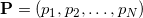
  (initially empty). In line with the sets and you can put a set of vectors
  and
and  . To do this, we mentally at every step of this algorithm choose any point
  from the set (db is not empty), remember it, then draw a vector from it to all the other points from (receiving at the same time which will contain less by one element than ) and to all points of (receiving ). First, take the first (or any other) point from and move it to . Next, look for a vector from with the largest module and move the corresponding point from at . The first point from move back to (it was chosen without any criteria). On each of the following steps looking for a point
  of which is as far as possible from affine space with a basis and move it from at . To do this, look for the corresponding point. vector
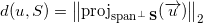
  of whose projection module on the orthogonal complement
  vector subspace
  max. Here - linear shell , that is, the vector space, since vector in are linearly independent (by construction), then - the basis of this vector space.
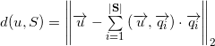
Formula distance from before :
Since the vector is directly decomposed into a sum of projections onto any subspace and onto the orthogonal complement of this subspace, then:

Having an orthonormal basis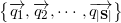 vector subspace , we can calculate the module of the projection onto the orthogonal complement of this subspace:
Coordinates of vectors we can get by performing a QR decomposition of a rectangular matrix (for example, using the Householder method) composed of (coordinates) column-vectors from the set . As a result, we obtain an orthogonal (rectangular) matrix Q (
  ) and upper triangular R (not used). The Q columns are the coordinates of the vectors. forming an orthonormal basis of a vector space .
After completing the algorithm in located point.
Two lists of points are kept: source list
(initially it contains all points from the input of the algorithm) and a list of points of the simplex (initially empty). In line with the sets and you can put a set of vectors and . To do this, we mentally at every step of this algorithm choose any point from the set (db is not empty), remember it, then draw a vector from it to all the other points from (receiving at the same time which will contain less by one element than ) and to all points of (receiving ). First, take the first (or any other) point from and move it to . Next, look for a vector from with the largest module and move the corresponding point from at . The first point from move back to (it was chosen without any criteria). On each of the following steps looking for a point of which is as far as possible from affine space with a basis and move it from at . To do this, look for the corresponding point. vector of whose projection module on the orthogonal complement vector subspace max. Here - linear shell , that is, the vector space, since vector in are linearly independent (by construction), then - the basis of this vector space.Formula distance from
before :Since the vector is directly decomposed into a sum of projections onto any subspace and onto the orthogonal complement of this subspace, then:
Having an orthonormal basis
vector subspace , we can calculate the module of the projection onto the orthogonal complement of this subspace:Coordinates of vectors
we can get by performing a QR decomposition of a rectangular matrix (for example, using the Householder method) composed of (coordinates) column-vectors from the set . As a result, we obtain an orthogonal (rectangular) matrix Q ( ) and upper triangular R (not used). The Q columns are the coordinates of the vectors. forming an orthonormal basis of a vector space .After completing the algorithm in
located point.Next, we must distribute the remaining points to the so-called lists of external points (outside sets) of the faces - these are lists of points that are maintained for each face and which are still not considered (hereinafter - unassigned, English unassigned) points that are relatively face planes on the other side than the interior of the simplex (or a temporary polyhedron in the future). Here we use the property of a convex polyhedron (and simplex in particular) that it lies entirely in only one of the two half-spaces obtained by splitting the whole space with the plane of each face. From this property follows the fact that if a point does not fall into any of the lists of external points of the faces of the convex hull, then it is reliably located inside it. In the future, the algorithm will need information about which of the points contained in the list of external points and the most distant from the plane of the face, therefore, adding points to the list of external points, you need to save information about which one is the furthest. Any point falls only in one list of external points. The asymptotic complexity is not affected by how exactly the points are distributed among the lists.
At this stage, I need to digress and tell how to set the face, how to calculate the distance to it, how to determine the orientation of a point relative to the face.
The brink. Oriented distance from the plane of the face to the point.
To set the brink we need to have points - vertices of the face. For the reasons given above, we will keep these points in an orderly manner. Moreover, the orderliness we need is not absolutely strict. For example, having made two exchanges in any two not necessarily different pairs of pairs of different points, we will get the same oriented edge in the sense that in any operations later (and this will usually be taking determinants from matrices formed from constants and coordinates of the vertices) such pair permutations do not affect the result. Two possible orientations correspond to two possible directions of the normal to the plane (face).
Only once - at the very beginning - we need to calculate the value of the hyper volume of the starting simplex in order to determine its orientation by a sign. All further operations regarding the edges will consist only in the calculation of the oriented distance (born distance) to the point. Here we can recall a school formula allowing generalization to the case of an arbitrary dimension, namely: “the area of a triangle is equal to half the product of the base, to a height” or “the volume of the pyramid is equal to one third of the product of the base to the height”. We are able to stretch the measure of the body and the face, therefore we can express the height (one-dimensional length):

In the algorithm, we need to calculate the oriented distance from a fixed plane (face) to points, which can be many. In this case, we can note that there is a positive constant in the denominator. From the position of the point ("above" or "under") depends only the hyper volume in the numerator. - also constant. Thus, we can consider only the relative values of the hyper-volumes of the simplexes (or rather, the corresponding parallelotopes) constructed from the face and the point. If the determinant is not considered the slowest way (by definition for  ) and not the fastest (
  ), and in the way through LUP decomposition (English LUP decomposition), it is possible to achieve complexity
 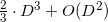 and decent numerical stability (born numerical stability). I do not undertake to evaluate how the complexity of calculating the determinant affects the final complexity of the entire algorithm, but experimenting, I concluded that in the worst case (for example, the case of points located on a sphere (English cospherical points)) even for small dimensions of space (
  ) calculating determinants to estimate distance is too computationally expensive.
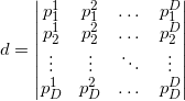
Another approach is to use the normalized plane equation (English hyperplane equation). This equation of the first degree, which relates the coordinates of a point of the plane, the coordinates of the normalized normal vector
 (
( 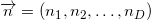 — ) (. normalized normal vector)
  (. offset):
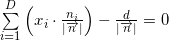
:
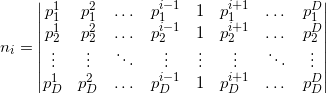
— :
, , — :

, , , — .
, — .
 and
and 
 - () .
: . std::inner_product , , , —  . , , , , , .
points - vertices of the face. For the reasons given above, we will keep these points in an orderly manner. Moreover, the orderliness we need is not absolutely strict. For example, having made two exchanges in any two not necessarily different pairs of pairs of different points, we will get the same oriented edge in the sense that in any operations later (and this will usually be taking determinants from matrices formed from constants and coordinates of the vertices) such pair permutations do not affect the result. Two possible orientations correspond to two possible directions of the normal to the plane (face).Only once - at the very beginning - we need to calculate the value of the hyper volume of the starting simplex in order to determine its orientation by a sign. All further operations regarding the edges will consist only in the calculation of the oriented distance (born distance) to the point. Here we can recall a school formula allowing generalization to the case of an arbitrary dimension, namely: “the area of a triangle is equal to half the product of the base, to a height” or “the volume of the pyramid is equal to one third of the product of the base to the height”. We are able to stretch the measure of the body and the face, therefore we can express the height (one-dimensional length):
In the algorithm, we need to calculate the oriented distance from a fixed plane (face) to points, which can be many. In this case, we can note that there is a positive constant in the denominator. From the position of the point ("above" or "under") depends only the hyper volume in the numerator.
- also constant. Thus, we can consider only the relative values of the hyper-volumes of the simplexes (or rather, the corresponding parallelotopes) constructed from the face and the point. If the determinant is not considered the slowest way (by definition for ) and not the fastest ( ), and in the way through LUP decomposition (English LUP decomposition), it is possible to achieve complexity and decent numerical stability (born numerical stability). I do not undertake to evaluate how the complexity of calculating the determinant affects the final complexity of the entire algorithm, but experimenting, I concluded that in the worst case (for example, the case of points located on a sphere (English cospherical points)) even for small dimensions of space ( ) calculating determinants to estimate distance is too computationally expensive.Another approach is to use the normalized plane equation (English hyperplane equation). This equation of the first degree, which relates the coordinates of a point of the
plane, the coordinates of the normalized normal vector ( — ) (. normalized normal vector) (. offset): : — : , , — :, ,
, — . and - () . : . std::inner_product , , , — . , , , , , .Now we are able to describe the face plane, but there is one ambiguity: how to choose the order of listing points in the lists of vertices of faces of the starting simplex? Authors do not keep the list of vertices ordered. They act differently. By setting the plane equation for an arbitrary but fixed order of the vertices, they find out the orientation of an internal point relative to this plane. That is, the oriented distance is calculated. If the distance is negative, they change the sign of the coordinates of the normal to the hyperplane and its offset from the origin. Or set the value of the flag, indicating that the face is inverted (English flipped). The internal point for a convex polyhedron will be the arithmetic average of at least
its vertices (the so-called center of mass, if we take all the vertices).Reorientation of the faces of the starting simplex.
( ) . , , (  ) (
) (  ). , «»
  , ( ). ,
  (
(  ). .
). .
 . , , . , . ( / ).
, , , , . , .
) ( ). , «» , ( ). , ( ). . . , , . , . ( / )., ,
, , . , .For each face, in addition to specifying a list of vertices, a list of external points, you must specify a list of adjacent (eng. Adjacency list) faces. For each face it will contain exactly
items.Since the starting simplex contains a face, it is obvious that for any of its faces, all other faces ( pieces) will fall into the list of adjacent faces .The main loop.
Now there is a temporary polygon with which you can work in the main loop. In the main cycle, this temporary polygon is completed by “capturing” more and more space, and with it the points of the original set, until a moment comes when there will not be a single point outside the polyhedron. Further I will describe this process in more detail. Namely, the way it works in my implementation.
The main loop is a loop along edges. At each iteration, among the faces with non-empty lists of external points, the best face is selected
(eng. Best facet); best in the sense that the farthest point from the list of external points is farther from the face than other faces. The cycle ends when there are no faces with non-empty lists of external points.In the body of the main loop, the selected face is deleted as a convex hull that is not the face of a convex hull. But beforehand, she "understands the components." From the list of external points, the farthest point is extracted
(eng. Furthest point) - it is probably the top of the convex hull. The remaining points are moved to a separate temporary list of unassigned points. .Further, according to the lists of adjacent faces, starting from the list of faces , the adjacency graph of the faces of the temporary polyhedron is bypassed and each face is added to the list of already visited (eng. Visited) faces and tested for visibility (eng. Visibility) from a point .If the face is invisible from a point , then its adjacent faces will not be further circumvented, otherwise they are bypassed. If the next visible face among neighboring faces has invisible ones from a point , then it falls into the list of border visible faces (the English before-the-horizon, as opposed to over-the-horizon, is “over the horizon”). But if all adjacent faces are visible, then such a face is added to the list of faces to be deleted. After traversing the adjacency graph of faces, the list of boundary visible faces and the list of faces to be deleted all contain all visible from the point.facets. Now all faces are deleted from the list for deletion. Moreover, each deleted face is not removed from the lists of neighboring faces from its neighbors. It is safe to do so, because even if the neighboring face is the visible edge of the border, from the list of its neighboring faces only information about the proximity to the invisible from the point is used in the future . Following the list of faces to be deleted is a list of visible edges. Each boundary visible edge is “parsed” (then we will need its list of adjacent faces and a list of vertices) and is deleted. For each boundary visible face, new faces are created (from one topieces), which are added to the list of new faces. At the same time, a list of its neighboring faces is viewed, and for each face from this list, which is invisible, a common edge with a given visible boundary is searched for. The vertices common to the invisible and boundary visible edges (that is, the vertices of the common edge) are written out to the list of vertices of a new face, moreover in the order in which they are written in the list of vertices of the boundary visible face. The edge (eng. Horizon ridge), by the way, is part of the horizon of that part of the surface of the temporary polyhedron that is visible from the point . The only vertex of the visible boundary that does not belong to this edge is replaced by the point in the list of vertices of the new face, the rest of the vertices are the same as in the (ordered) list of vertices of the boundary visible face and stand in the same places. Thus, the constructed list of vertices of the new facet guarantees its correct orientation, that is, when calculating its normalized plane equation, the normal will be directed outside the time polyhedron and the offset value will receive the correct sign. After all the boundary visible edges are processed, we have a list of new faces. The hyperplane equations for these faces can be calculated immediately after we have vertex lists for them. Also, when creating new faces, one can add one facet to their lists of adjacent faces, namely, the corresponding invisible face that was adjacent to the boundary visible face when forming the list of vertices of a new face. Obviously the restNeighboring faces must be searched for among other new faces.As it turned out (when sampling by the profiler from Google Performance Tools ), the most time in the case of large dimensions and / or poor input data (that is, when most of the points are vertices of a convex hull) the algorithm spends searching for neighboring faces for new faces. In my implementation, the algorithm was initially very simple: all possible pairs (two nested loops) of faces from the list of new faces were searched and comparisons were made (by the number from the input list of points) of vertex lists with one mismatch (modified algorithm std :: set_difference or std :: set_symmetric_difference ). I.e
comparisons, where - the number of new faces. But later I managed to win a pair (binary =) orders in the speed of searching for neighboring ones using ordered associative arrays ( std :: set ) in this narrow place. In general, there is a whole area of knowledge that is associated with this task (identifying neighbors) - this is locality-sensitive hashing . In the original implementation of qhulljust hashes are used (not LSH). It contains a separate data structure for each edge (two faces) (a list of edge vertices and information about faces “above” and “below” an edge), each face contains a list of its edges. To determine the neighborhood of the faces (among the faces from the list of new faces) for all edges of the faces, an associative unordered array of hashes of arrays of their vertices is created (with one skip (English skip) and one dropped vertex ). I.e saves hashes. If there is a collision (and the subsequent complete coincidence of the lists) of hashes, then (obviously) these two faces have a common edge (the hash, by the way, can be removed to reduce the hash table) and each of them can be added to the list of adjacent faces of the other. I do not use this method, since neither in the standard library nor in the STL there is such a tool as hash combiner (upd. Received information that the best choice is just XOR). I didn’t want to specialize without the information-theoretical justification of the correctness of std :: hash for std :: vector <std :: size_t> . That is why I used associative orderededge container for finding adjacent faces. As a result (apparently) my implementation of the algorithm loses qhull in speed asymptotically in from before times (for all sorts of input data).Comparative testing.
The example is the “canonical” implementation of the Quickhull qhull algorithm, installed through the package manager (in Ubuntu 14.04 LTS). To generate input from the same qhull-bin package, the rbox utility was used . The rbox tn D4 30000 s> /tmp/qhuckhull.txt command creates a file with coordinates of 30,000 points on a four-dimensional sphere. The rbox tn D10 30 s> /tmp/quickhull.txt command creates a file with the coordinates of 30 points on a ten-dimensional sphere. The amount of memory that the program spends can be seen in the output of the / usr / bin / time utility with the -v option . Thus, in the output / usr / bin / time -v bin / quickhull /tmp/quickhull.txt | head -7 you can find out the consumption of both memory and processor time (cleared from the time to read files and output to the terminal) for my implementation, and in the output / usr / bin / time -v qconvex s Qt Tv TI /tmp/quickhull.txt - for the “canonical” implementation of qhull .
I determine the correctness of my implementation by the coincidence of the number of faces of the convex hulls. But for debugging (in two-dimensional and three-dimensional modes) at some stage I implemented step-by-step (via the pause command) animated output in gnuplot format. Somewhere in commits it is. The output of the program is a convex hull and a numbered set of input points represented in the gnuplot format.
In addition, somehow I started writing (but did not finish) the randombox utility, an analogue of rbox . randombox was conceived as a utility that generates points uniformly distributed in space (English uniform spatial distribution), in contrast to rbox , which generates points that are not evenly distributed. randombox can generate sets of points bounded by a simplex (of any dimension that can be embedded in space with points), on a unit sphere (in the unit sphere), in a ball (English ball), on the surface of a single “diamond-shaped” polyhedron (Eng. unit diamond), inside a unit cube (English unit cube), inside a parallelotope, within the standard unit simplex (English unit simplex), and also projects a set of points into the volume of the cone (English cone) or cylinder (English cylinder ). To generate coordinates that are evenly distributed within an arbitrary speclex (embedded in space), I found a numerically stable algorithm on the Internet (through the Dirichlet distribution), and also came up with my own algorithm, which does not have this property. In the end, chose the first.
In order to “feel” the bulging shells with a glance using gnuplot , from the project root enter the command rbox n D3 40 t | bin / quickhull> /tmp/quickhull.plt && gnuplot -p -e "load '/tmp/quickhull.plt'" . rbox n D3 40 t will generate 40 points inside the bounding cube
(eng. bounding box). The key t specifies the use of the current time (in seconds) as the initial PRNG value. To get points on a sphere, you need to add the key s . It is also interesting to see how nonsimplicial faces are broken: rbox n D3 c - cube, rbox n D3 729 M1,0,1 - points located in whole nodes. The convex shell of the helix looks beautiful (eng. Helix): rbox n D3 50 l . In the case of the simultaneous location of a large number of points coplanar to the edges, the constant eps begins to play a great role for the correctness of the results, which is set when constructing the algorithm object. For example, if you use std :: numeric_limits <value_type> :: epsilon () as a small value, then in the case of a “rotated” cube of 64 integer points of rbox n D3 64 M3.4, as a result of the algorithm, an incorrect which is a convex polygon.Total or late TL; DR.
The result of my work was the release of the Quickhull algorithm in C ++, quite compact and not very slower than the implementation with qhull.org . The algorithm receives at the input the value of the dimension of space, the value of the small constant eps and the set of points represented as a range defined by a pair of iterators, as is customary in STL. At the first stage of create_simplex, the starting simplex is built and the point basis of the affine (sub) space containing the input points is returned. If the number of points in the basis is greater than the dimension of the Euclidean space containing the points, then the algorithm for completing the construction of the convex hull must be run. At the output, the algorithm will give an array of data structures describing the faces of the convex hull of the input set, which is the answer. In case of failure, we have a point basis of some subspace of lower dimension, which contains all points. Using the Householder algorithm, you can in some way rotate the input set, while vanishing the highest coordinates of the points. Such coordinates can be discarded and the Quickhull algorithm can be applied already in a space of lower dimension.
Applications.
This algorithm has many applications. In addition to finding the convex hull as such, due to the fact that there is a connection between the convex hull , the Delaunay triangulation and the Voronoi diagram , it is easy to find applications of the algorithm "indirectly".
This implementation has already come in handy for some people , and was paid for with gratitude (in Acknowledgments), which is very nice.
Updates.
06/24/2015: A check of the convexity of the resulting geometric structure was added according to the algorithm of Kurt Mehlhorn, Stefan Näher, Thomas Schilz, Stefan Schirra, Michael Seel, Raimund Seidel, and Christian Uhrig. Checking geometric programs or verification of geometric structures. In Proc. 12th Annu. ACM Sympos. Comput. Geom., Pages 159-165, 1996 .
06/24/2015: The faces of the resulting polyhedron now contain sets of vertices and indices of neighboring faces arranged in such a way that the face is the opposite one and the corresponding vertex. This makes the structure much more convenient to use in some cases.
06.24.2015 G .: Now for the determination of the neighborhood of newly obtained faces, their hashes are used.
Source: https://habr.com/ru/post/245221/
All Articles