Lagrange formalism in problems with dry friction

Introduction

This article is a logical continuation of the topic begun in the previous publication . As promised in the comments, we consider the applicability of the method of redundant coordinates to the dynamic analysis of mechanical systems moving under the action of dry Coulomb friction forces. As an illustrative example, solve the following problem

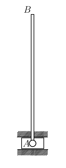
A thin homogeneous mass rod m = 2 kg, length AB = 2 l = 1 m at point A is pivotally attached to a weightless slider moving in horizontal rough guides. At the initial moment of time, the rod is located vertically, then it is deflected from the vertical at a negligibly small angle and released without the initial velocity. It is necessary to make up the equations of motion of a given mechanical system and find the law of its motion. The friction coefficient between the slider and the guides is equal to f = 0.1.

')
Before proceeding to the solution of the problem by the method proposed by the author, we consider a slightly elementary theory concerning dry friction.

1. What could be "easier" friction?

There is no more terrible punishment for a mechanic than friction force. Appearing in the problem, this force immediately makes it essentially nonlinear, because it behaves in a rather interesting way.

Consider a fairly simple example. Let a horizontal bar rest on a rough surface.

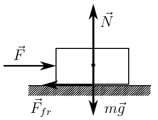
Let no force be applied to it at the beginning (except for gravity and normal reaction). In this case, the friction force between the bar and the plane will be zero.

Now apply a small horizontal force to the bar. The bar will not budge, since in response to our impact from the surface, a friction force will act on it, which will satisfy the condition

$\ vec {F} _ {fr} = - \ vec {F} \ quad \ quad (1)$

We will gradually increase the strength $\ vec {F}$ and, according to (1), the friction force will also grow, which in this case is called the friction force of rest . This will continue until the friction force of rest reaches the value

$F_ {fr} ^ {\ max} = fN$

called the limit value of the friction force of rest. Here f is the coefficient of dry friction between the bar and the plane; N is a normal reaction from the plane. After that, the friction force will cease to grow, and with a further increase in the horizontal force, the bar will begin to slip. The frictional force will translate into a sliding friction force equal to

$\ vec {F} _ {fr} = -fN \ cfrac {\ vec {v}} {\ left | \ vec {v} \ right |} \ quad \ quad (2)$

Where $\ vec {v}$ - the speed of the bar.

The example is rather trivial, but it reveals the essence of the behavior of the dry friction force. Thus, we obtain the following algorithm for calculating the friction force:

If the point where the applied friction force is fixed:

Calculate the friction force of rest and normal reaction
Check condition
$F_ {fr} \ le fN$
in violation of which we accept the friction force equal to the ultimate friction force of rest

If the point of application of the friction force moves:

Calculate the normal reaction
Calculate the force of sliding friction, according to the expression (2)

2. Simulation of motion systems with friction

Now we solve our problem. The system we are considering has two degrees of freedom, but because of the need to determine the normal reaction, we expand the number of degrees of freedom to three and obtain the following calculation scheme

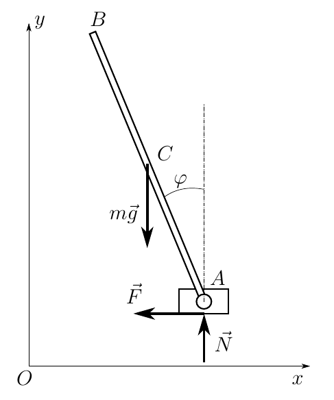
Here we take the vector as generalized coordinates.

$\ vec {q} = \ left [x (t), y (t), \ varphi (t) \ right] ^ T \ quad \ quad (3)$

where x, y are the coordinates of point A ; $\ varphi$ - the angle of the rod to the vertical. Arming Maple'om

#   restart; #    with(LinearAlgebra): #    read `/home/maisvendoo/work/maplelibs/mechanics/lagrange.m`:

We determine the kinematics of the system

 #    q := [x(t), y(t), phi(t)]: #   A xA := q[1]: yA := q[2]: #     xC := q[1] - L*sin(q[3]): yC := q[2] + L*cos(q[3]): # -  A  C rA := Vector([xA, yA]): rC := Vector([xC, yC]): #      VectorCalculus[BasisFormat](false): vC := VectorCalculus[diff](rC, t):

Calculate its kinetic energy

 #       J := m*(2*L)^2/12: #    T := simplify(J*diff(q[3], t)^2/2 + m*DotProduct(vC, vC, conjugate=false)/2);

Maple produces this result.

$T = 1/6 \, m \ left (4 \, {L} ^ {2} \ left ({\ frac {d} {dt}} \ phi \ left (t \ right) \ right) ^ {2} -6 \, L \ left ({\ frac {d} {dt}} \ phi \ left (t \ right) \ right) \ left ({\ frac {d} {dt}} x \ left (t \ right ) \ right) \ cos \ left (\ phi \ left (t \ right) \ right) -6 \, L \ left ({\ frac {d} {dt}} \ phi \ left (t \ right) \ right ) \ left ({\ frac {d} {dt}} y \ left (t \ right) \ right) \ sin \ left (\ phi \ left (t \ right) \ right) +3 \, \ left ({ \ frac {d} {dt}} x \ left (t \ right) \ right) ^ {2} +3 \, \ left ({\ frac {d} {dt}} y \ left (t \ right) \ right) ^ {2} \ right)$

It is rather cumbersome, but we don’t “pick” with our hands on a piece of paper, so we move on. We set vectors and points of application of forces

 #  ,    Mg := Vector([0, -m*g]): #   F_A := Vector([-F, 0]): #   N_A := Vector([0, N]): #   #    Fk := [Mg, F_A, N_A]: #      rk := [rC, rA, rA]:

We obtain the equations of motion of the system in the form of Lagrange 2 kind

 #    2  EQs := LagrangeEQs(T, q, rk, Fk):

We get three "crocodiles"

$\ frac {4} {3} mL ^ 2 \ ddot {\ varphi} -mL \ ddot {y} \ sin \ varphi-mL \ ddot {x} \ cos \ varphi = mgL \ sin \ varphi \ quad \ quad ( four)$

$m \ ddot {y} -mL \ dot {\ varphi} ^ 2 \ cos \ varphi - mL \ ddot {\ varphi} \ sin \ varphi = N - mg \ quad \ quad (5)$

$m \ ddot {x} + mL \ dot {\ varphi} ^ 2 \ sin \ varphi-mL \ ddot {\ varphi} \ cos \ varphi = -F \ quad \ quad (6)$

These equations had to be hammered into the article with my hands, because Maple's “copy-paste” of LaTeX output leads to an unattractive result. But even this can be seen - the equations are complex and given the fact that F is the friction force, they are not analytically integrable.

Now we introduce the equation of relations. First, the slider moves along horizontal guides, therefore

$y (t) = 0 \ quad \ quad (7)$

In addition, in the case when the slider is stationary and the friction force at rest does not exceed the limit value, one more connection is activated

$x (t) = A \ quad \ quad (8)$

Where $A = \ text {const}$ - some horizontal coordinate of the slider. Now we transform the system (4) - (6) taking into account equations (7) and (8) and find the friction force of rest and the normal reaction

 #   link_eq1 := q[1] = A: #  ,    -    link_eq2 := q[2] = 0: #     X Link_EQs := {link_eq1, link_eq2}: #           Reduced_EQs := ReduceSystem(EQs, Link_EQs, q): solv_reduced := SolveAccelsReacts(Reduced_EQs, [q[3]], [F, N]): #     for i from 1 to numelems(solv_reduced) do if has(solv_reduced[i], F) then F1 := rhs(solv_reduced[i]); end if; if has(solv_reduced[i], N) then N1 := rhs(solv_reduced[i]); end if; end do:

Here I will give the result directly issued Maple

$F_1 = -mL \ sin \ left (\ phi \ left (t \ right) \ right) \ left ({\ frac {d} {dt}} \ phi \ left (t \ right) \ right) ^ {2} +3/4 \, \ cos \ left (\ phi \ left (t \ right) \ right) mg \ sin \ left (\ phi \ left (t \ right) \ right) \ quad \ quad (9)$

$N_1 = -mL \ cos \ left (\ phi \ left (t \ right) \ right) \ left ({\ frac {d} {dt}} \ phi \ left (t \ right) \ right) ^ {2} -3/4 \, \ left (\ sin \ left (\ phi \ left (t \ right) \ right) \ right) ^ {2} mg + mg \ quad \ quad (10)$

If you look at the resulting expressions, they are quite consistent with the logic of the process. Now we obtain an expression for calculating the normal reaction in the case when the slider slides along the guides, taking into account that in this case the friction force will be determined by the expression

$F = fN \ text {sign} \ left (\ dot {x} \ right)$

(minus is already in the equations of motion)

 #          Slade_EQs := ReduceSystem(EQs, {link_eq2}, q): #        for i from 1 to numelems(Slade_EQs) do Slade_EQs[i] := subs(F = f*N*signum(diff(q[1], t)), Slade_EQs[i]); end do: solv_slade := SolveAccelsReacts(Slade_EQs, [q[1], q[3]], [N]): #      for i from 1 to numelems(solv_reduced) do if has(solv_slade[i], N) then N2 := rhs(solv_slade[i]); end if; end do:

Hmmm, the crocodile is still out, especially since Maple does generate enough LaTeX code

$N_2 = - {\ frac {m \ left (3 \, L \ left ({\ frac {d} {dt}} \ phi \ left (t \ right) \ right) ^ {2} \ left (cos \ left (\ phi \ left (t \ right) \ right) \ right) ^ {3} +3 \, L \ left ({\ frac {d} {dt}} \ phi \ left (t \ right) \ right ) ^ {2} \ cos \ left (\ phi \ left (t \ right) \ right) \ left (\ sin \ left (\ phi \ left (t \ right) \ right) \ right) ^ {2} - 4 \, L \ cos \ left (\ phi \ left (t \ right) \ right) \ left ({\ frac {d} {dt}} \ phi \ left (t \ right) \ right) ^ {2} -3 \, \ left (\ cos \ left (\ phi \ left (t \ right) \ right) \ right) ^ {2} g-3 \, \ left (\ sin \ left (\ phi \ left (t \ right) \ right) \ right) ^ {2} g + 4 \, g \ right)} {3 \, f \ sin \ left (\ phi \ left (t \ right) \ right) \ cos \ left ( \ phi \ left (t \ right) \ right) {\ it \ text {sign}} \ left ({\ frac {d} {dt}} x \ left (t \ right) \ right) +3 \, \ left (\ cos \ left (\ phi \ left (t \ right) \ right) \ right) ^ {2} -4}} \ quad \ quad (11)$

All the expressions we need are obtained, now we can proceed to modeling. In contrast to the problem with a pendulum, about which I have already written, here we honestly transform our equations with Maple-means for a form suitable for a numerical solution. First of all, we solve equations (4) - (6) with respect to generalized accelerations

 #        Main_EQs := SolveAccelsReacts(EQs, q, []): #    s := numelems(q):

I will not give the result anymore - it is also quite cumbersome. Go to the phase coordinates

 #    # Y[1] -> x(t) # Y[2] -> y(t) # Y[3] -> phi(t) # Y[4] -> vx(t) -     # Y[5] -> vy(t) -     # Y[6] -> omega(t) -    #            for i from 1 to s do N2 := subs(diff(q[i], t) = y[i+s], N2); N2 := subs(q[i] = y[i], N2); N1 := subs(diff(q[i], t) = y[i+s], N1); N1 := subs(q[i] = y[i], N1); F1 := subs(diff(q[i], t) = y[i+s], F1); F1 := subs(q[i] = y[i], F1); end do: #        for i from 1 to s do for j from 1 to s do eq := Main_EQs[j]; if has(eq, diff(diff(q[i], t), t)) then accel[i] := rhs(eq); end if; end do; for j from 1 to s do accel[i] := subs(diff(q[j], t) = y[j+s], accel[i]); accel[i] := subs(q[j] = y[j], accel[i]); end do: end do:

We form the functions of calculating the forces we need

 #       GetN1 := proc(mass, length, grav_accel, fric_coeff, Y) local react := subs(m = mass, L = length, g = grav_accel, f = fric_coeff, N1); local i; for i from 1 to numelems(Y) do react := subs(y[i] = Y[i], react); end do: return evalf(react); end proc: #       GetN2 := proc(mass, length, grav_accel, fric_coeff, Y) local react := subs(m = mass, L = length, g = grav_accel, f = fric_coeff, N2); local i; for i from 1 to numelems(Y) do react := subs(y[i] = Y[i], react); end do: return evalf(react); end proc: #     GetF1 := proc(mass, length, grav_accel, fric_coeff, Y) local react := subs(m = mass, L = length, g = grav_accel, f = fric_coeff, F1); local i; for i from 1 to numelems(Y) do react := subs(y[i] = Y[i], react); end do: return evalf(react); end proc:

The code given, albeit voluminous, is quite simple - the substitution of numerical parameters into the corresponding expressions and their calculation is performed. We form the same function to calculate generalized accelerations.

 #     GetAccel := proc(mass, length, grav_accel, fric_force, normal_react, Y) local acc; local i, j; for i from 1 to numelems(Y)/2 do acc[i] := subs(m = mass, L = length, g = grav_accel, F = fric_force, N = normal_react, accel[i]); end do: for i from 1 to numelems(Y)/2 do for j from 1 to numelems(Y) do acc[i] := evalf(subs(y[j] = Y[j], acc[i])); end do: end do: return [seq(acc[i], i=1..numelems(Y)/2)]; end proc:

We set the parameters given to us in the statement of the problem

 #    m1 := 2.0; L1 := 0.5; f1 := 0.1; g1 := 9.81;

Time to set the basic logic of the model, which determines the calculation of the friction force. In this case, we set the error of the speed of the slider, at which we will consider it equal to zero.

 #       GetFricNormal := proc(mass, length, grav_accel, fric_coeff, Y) local F1, N1; #      local eps_v := 1e-6; #     #    if abs(Y[4]) < eps_v then #        F1 := GetF1(mass, length, grav_accel, fric_coeff, Y); N1 := GetN1(mass, length, grav_accel, fric_coeff, Y); #       , #        if abs(F1) > fric_coeff*abs(N1) then F1 := fric_coeff*abs(N1)*signum(F1); end if; else #    ,       N1 := GetN2(mass, length, grav_accel, fric_coeff, Y); F1 := fric_coeff*abs(N1)*signum(Y[4]); end if; return [F1, N1]; end proc:

Define a callback for the solver:

 #           (  ) EQs_func := proc(N, t, Y, dYdt) local F1, N1; #      local acc; #   local ret; #       ret := GetFricNormal(m1, L1, g1, f1, Y); F1 := ret[1]; N1 := ret[2]; #     acc := GetAccel(m1, L1, g1, F1, N1, Y); dYdt[1] := Y[4]; dYdt[2] := Y[5]; dYdt[3] := Y[6]; dYdt[4] := acc[1]; dYdt[5] := acc[2]; dYdt[6] := acc[3]; end proc:

We form the list of phase coordinates for the solver and the initial conditions (the bar deflection angle from the vertical is made small) and perform numerical integration (in fact, the last dsolve () call only indicates our intentions by a numerical solution - it will be produced when calculating specific values of phase coordinates).

 #    vars := [X(t), Y(t), Phi(t), Vx(t), Vy(t), Omega(t)]; #   initc := Array([0.0, 0.0, 1e-4, 0.0, 0.0, 0.0]); #   dsolv := dsolve(numeric, number = 6, procedure = EQs_func, start = 0, initial = initc, procvars = vars, output=listprocedure);

Perform some preparatory operations

 #      x := eval(X(t), dsolv); y := eval(Y(t), dsolv); phi := eval(Phi(t), dsolv); vx := eval(Vx(t), dsolv); vy := eval(Vy(t), dsolv); omega := eval(Omega(t), dsolv);

Next, we calculate the motion of the system for a certain time interval and form arrays of data for output to the graphs

 #         t0 := 0.0: t1 := 10.0: num_plots := 1000: dt := (t1 - t0)/num_plots: t := t0: i := 1: while t <= t1 do Time[i] := t; Y := [x(t), y(t), phi(t), vx(t), vy(t), omega(t)]; x1[i] := Y[1]; phi1[i] := Y[3]; fric[i] := GetFricNormal(m1, L1, g1, f1, Y)[1]; norm_react[i] := GetFricNormal(m1, L1, g1, f1, Y)[2]; lim_fric[i] := f1*abs(norm_react[i])*fric[i]/abs(fric[i]); t := t + dt; i := i + 1; end do:

Well, we have almost everything ready

 #   G_x := [ [Time[k],x1[k]] $k=1..num_plots]: G_phi := [ [Time[k],phi1[k]] $k=1..num_plots]: G_fric := [ [Time[k],fric[k]] $k=1..num_plots]: G_norm_react := [ [Time[k],norm_react[k]] $k=1..num_plots]: G_lim_fric := [ [Time[k],lim_fric[k]] $k=1..num_plots]: #     gr_opts := captionfont=['ROMAN', 16], axesfont=['ROMAN','ROMAN', 12],titlefont=['ROMAN', 14],gridlines=true: plot(G_x, gr_opts, view=[t0..t1, -1..1.0]); plot(G_phi, gr_opts, view=[t0..t1, 0.0..7.0]); plot({G_fric, G_lim_fric}, gr_opts, view=[t0..t1, -20..20]); plot(G_norm_react, gr_opts, view=[t0..t1, 0.0..200.0]);

We get graphics. Beauty for the sake of graphics were converted from Maple to * .eps and slightly processed in inkscape.

Move the slider

Rod deflection angle from vertical

Friction force

Here the blue line shows the limit value of static friction, and the red line shows the actual value of the friction force.

Normal reaction from guides

It can be seen that the slider rests for a little more than two seconds, and then, after overcoming the friction of rest, it begins to move, which gradually fades out and completely stops 6.5 seconds after the start of movement. After that, the friction force never exceeds the limit value for rest, the slider remains in place, and the rod performs harmonic oscillations around a stable equilibrium position.

Conclusion

The application of the method of redundant coordinates and Lagrange equations of the second kind to the analysis of the motion of systems with dry friction is considered. It can be seen that with the external bulkiness of the results obtained, the process of synthesis of the equations of motion can be automated by means of symbolic mathematics, and this is essential for modern technical tasks.

Thank you for your attention to my work.

Source: https://habr.com/ru/post/245211/

All Articles

Lagrange formalism in problems with dry friction

Introduction

1. What could be "easier" friction?

2. Simulation of motion systems with friction

Conclusion

More articles: