Angle detectors
I am interested in image processing, especially working with special points. Looking for information on angle detectors, I did not find a sufficiently large overview of these algorithms in Russian. Therefore, I decided to correct the situation by writing this article. The layout of the article is as follows:
')
In order to extract some interpreted information from an image, it is necessary to bind to local features of the image. On the image it is possible to highlight particular points A particular point m , or point feature (key point), an image is an image point whose neighborhood o (m) can be distinguished from the neighborhood of any other point of the image o (n) in some other neighborhood of the singular point o 2 (m) . For the majority of algorithms, a rectangular window measuring 5x5 pixels is taken as the neighborhood of the image point. The process of determining the singular points is achieved by using a detector and a descriptor.
A detector is a method of extracting specific points from an image. The detector ensures the invariance of finding the same singular points with respect to image transformations.
Descriptor is an identifier of a singular point that distinguishes it from the rest of the set of singular points. In turn, descriptors should ensure the invariance of finding a correspondence between specific points with respect to image transformations [1].
In 1992, Haralick and Shapir [10] identified the following requirements for particular points as the following properties:
Interestingly, in [5], Tuytelaars and Mikolajczyk (2006) identified the following properties that particular points should have:
In general, these properties intersect with [10], but are interpreted differently.
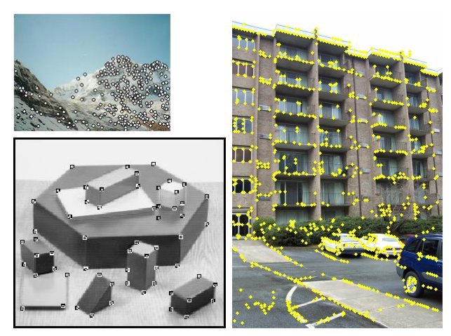
There are many algorithms for determining the special points, designed for different applications. In this article, I pay attention to angle detectors (or how they are called corner detector).
Angles (corners) are particular points that are formed from two or more faces, and faces usually define the boundary between different objects and / or parts of the same object. [2] In another way, we can say that the angles are the point at which in the neighborhood the intensity varies relative to the center (x, y) . Angles are determined by coordinates and changes in the brightness of the surrounding points of the image. The main property of such points is that in the area around the corner of the image gradient two dominant directions prevail, which makes them distinguishable. Gradient is a vector quantity that indicates the direction of the steepest increasing of the image intensity function I (x, y) . Since the image is discrete, the gradient vector is determined through the partial derivatives along the x and y axes through changes in the intensities of the adjacent image points. Most methods consider angularity depending on a derivative of the 2nd order, therefore, in general, methods are sensitive to noise.
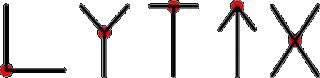
Depending on the number of intersected faces, there are different types of angles: L-, Y- (or T-), and X- connected [3] (some still have swept-connected angles [2]). Different corner detectors react differently to each of these types of corners.
Approaches to the definition of singular points can be divided into 3 categories [10]:
In practice, methods based on image intensity are the most common for widespread use.
Next, I will consider descriptions of the main detectors of singular points defining angles. Then a comparative table of detectors will be presented with conclusions about their applicability to various situations and, finally, images with corner detectors applied to them.
Work in the study of image binding using singular points began the Moravec detector (Moravec, 1977). The Moravec detector is the simplest of all. The author considers the change in the brightness of a square window W (usually 3x3, 5x5, 7x7 pixels) relative to the point of interest when the window W is shifted by 1 pixel in 8 directions (horizontal, vertical and diagonal) [4]. Algorithm:
Moravec detector has anisotropy property in 8 directions of window displacement. The main disadvantages of the detector under consideration are the lack of rotation transformation invariance and the occurrence of detection errors in the presence of a large number of diagonal edges [2].
Studies have shown that the most optimal detector of L-connected angles is the well-known Harris detector (also called the Plessey operator, the Harris and Stephens detector, Plessey operator, Harris and Stephens detector, 1988) [5] [6].
Harris and Stephens improved the Moravec detector by introducing anisotropy in all directions, i.e. consider the derivatives of the brightness of the image to study changes in brightness in many directions. They introduce derivatives in some principal directions.
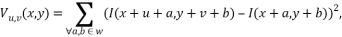
For this image I, consider the window W (usually the window size is 5x5 pixels, but may depend on the image size) in the center (x, y) , as well as its shift by (u, v) .

Then the weighted sum of squared differences (sum of squared differences (SSD)) between the shifted and initial window (i.e., the change in the neighborhood of the point (x, y) when shifted by (u, v) ) is equal to:

where w (x, y) is a weight function (usually a Gaussian function or a binary window is used).

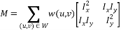
M - autocorrelation matrix:
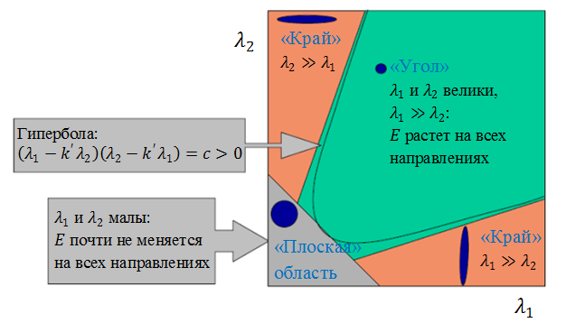
The angle is characterized by large changes in the function E (x, y) in all possible directions (x, y) , which is equivalent to the eigenvalues of matrix M that are large in modulus. The location of the eigenvalues is shown in the following figure.
Since it is a laborious task to directly consider eigenvalues, Harris and Stephen proposed a measure of response [7]:

where k is an empirical constant, .
.
Thus, the value of R is positive for angular singular points. Then the points are cut off by the found threshold R (i.e., those points for which the value of R is less than a certain threshold are excluded from consideration). Next are the local maxima of the response function (non-maximal suppression) over a neighborhood of a given radius and are selected as corner singular points.
The Harris detector is invariant to rotations, partially invariant to affine changes in intensity. The disadvantages include the sensitivity to noise and the dependence of the detector on the scale of the image (to eliminate this drawback, Harris's multi-scale detector is used).
The Shih-Tomasi angular detector (Shi-Tomasi or Kanade-Tomasi, 1993) largely coincides with the Harris detector, but differs in the calculation of the response measure: the algorithm directly calculates the value since the assumption is made that the search for angles will be more stable. The authors use the same equation to analyze the optical flux of Lucas and Canada (Lucas and Kanade). The details of the algorithm are given in [8] and [9].
Förstner and Gölch (Förstner and Gülch, 1987) were the first to describe a method that uses the same angularity measure as the Harris detector. They used a more complex computational implementation [8]. Unlike the Harris detector, the eigenvalues are computed explicitly. The response function of the Förstner angle is defined as follows:

Also for the correctness of the definition is considered a measure of the roundness of the angle, equal to: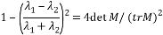 .
.
In practice, the Förstner detector is often used to extend the capabilities of the Harris detector — to find circular singular points along with the corners. Also, the algorithm has the best localization property [2].
A more detailed description of the algorithm is presented in Wikipedia , as well as in [10], [11].
The SUSAN (Smallest Univalue Segment Assimilation Nucleus) algorithm was proposed by Smith and Brady (Smith and Brady, 1997) [5].
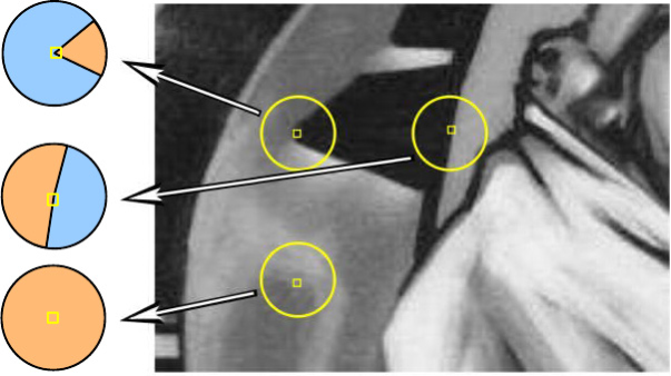
Angles are determined by segmentation of circular neighborhoods into similar (orange) and unlike (blue) areas. Angles are located where the relative area of similar areas (similar USAN) reaches a local minimum below a certain threshold.
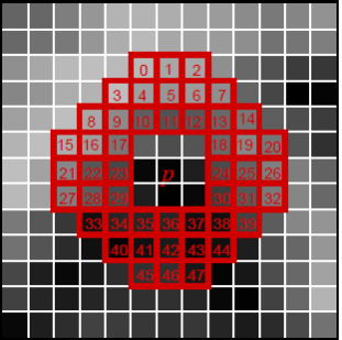
For each pixel, a circular area of fixed radius is considered. The center of the pixel is called the core, its intensity value is remembered. All other pixels are divided into 2 categories: similar (orange) and unlike (blue) areas, depending on whether the intensity of the core is similar or not. Where there is a section of the image under a circular area unchanged, similar areas occupy almost the entire area, on the edges this ratio drops to 50%, at the corners it decreases to about 25%. Thus, the angles are located where the relative area of similar areas (similar USAN) reaches a local minimum below a certain threshold. To increase the stability of the algorithm, the authors assign higher weights to the pixels closest to the core. The steps of the algorithm are as follows:
The algorithm shows good accuracy for all kinds of angles, but is not susceptible to blurring on images. Details are given in [12].
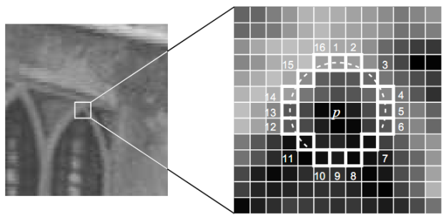
Tryakovits and Hedley (Miroslav Trajkovic and Mark Hedley, 1998) in the article “Fast corner detection” introduced a new type of detector - the operator Tryakovits [8]. Initially, the authors made demands on him to become the most popular angle detector and have the minimum computational cost. First, the 4-neighbor algorithm Trajkovic4 was developed.
The detector checks the area around the pixel by examining nearby pixels: let c be the pixel to be considered, and P be the point on the circle S N at the center at the point N. Point P ' is the point opposite to P in diameter.
Response functions (authors call it CRN, Corner Request Function) are defined as:

where N is the center point;
P and P ' are two points opposite in diameter around point N ;
S N - sampled circle on an image with a radius of 3, 5, 7 pixels.

The CRN value will be large when there is no direction in which the central pixel resembles two nearby pixels in diameter. Since the calculation in any direction gives an upper limit of min, the horizontal and vertical directions are checked first to determine whether it makes sense to move on to the full calculation of R N.
In comparison with the Harris detector, the frequency of repeatability of the Trajkovic4 algorithm is worse, but localization is comparable with the definition of L-connected angles and is superior to other types of angles.
Also, the disadvantages include the fact that this 4-neighbor operator falsely reacts to diagonal edges and is sensitive to noise [2]. Therefore, use the 8-connected version of this algorithm Trajkovic8. Trajkovic8 differs from Trajkovic4 in the way it calculates angularity. However, Trajkovic8 still finds false angles on some diagonal edges of the object (it does not show itself well on artificial images). Detailed descriptions of the algorithms are given in [2] and [8].
Rosten and Drummond (Edward Rosten and Tom Drummond, 2005) introduced a rather successful FAST algorithm (Features from Accelerated Segment Test) - features of the accelerated segment tests.
The algorithm considers a circle of 16 pixels (drawn by the Bresenham algorithm) around candidate point P. A point is angular if for the current considered point P there are N adjacent pixels on a circle whose intensities are greater than I P + t or the intensities of all are less than I P -t , where I P is the intensity of point P , t is a threshold value. Next, you need to compare the intensity at the vertical and horizontal points on the circle numbered 1, 5, 9 and 13 with the intensity at point P (in order to cut off the false candidates as quickly as possible). If the condition I Pi > I P + t or I Pi <I P + t, i = 1, .., 4 , is fulfilled for 3 of these points, then a complete test is performed for all 16 points [13]. Experiments have shown that the smallest value of N , at which singular points begin to be detected steadily, is N = 9 .
Initially, the original algorithm was FAST-12 . There are modifications of the algorithm: tree-like FAST-9 and FAST-12 (the tree based FAST-9 and FAST-12).
The original algorithm has several drawbacks, for example, several particular points can be found near a certain neighborhood, the efficiency of the algorithm depends on the order of image processing and the distribution of pixels.
In [14], the authors Edward Rosten, Reid Porter, and Tom Drummond (2008) introduce improvements to the FAST algorithm, namely, that they use machine learning to determine specific points.
This algorithm they called FAST-ER (ER - Enhanced Repeatability, improved repeatability). The algorithm is stable to the property of repeatability: on the same scene, viewed from different angles, there are special points belonging to the same objects.
This algorithm uses a ring of a circle of more than 1 pixel, rather than in FAST (48 pixels). The authors use the ID3 algorithm to classify special points (whether the candidate point is special) using decision trees. The ID3 algorithm optimizes the order in which pixels are processed, resulting in the most computationally efficient detector.
The cost function of the decision tree is calculated as follows:

R is a measure of repeatability;
N is the number of detected singular points;
S is the number of nodes in the decision tree.
Details are described in [14].
FAST-ER is better than FAST, but slower in execution speed. The authors concluded that the FAST-ER detector is the best in relation to the repeatability property.
Rattarangsi and Chin (1992) [15] proposed an algorithm based on curvature scale space (CSS) that detects angles on flat curves. CSS is suitable for extracting invariant geometric features on a flat curve at various scales.
The algorithm determines singular points using several scales of the same image. However, it is computationally complex and detects false angles in circular areas. [sixteen]
Farzin Mokhtarian and Riku Suomela (1998) [17] improved the algorithm in noise resistance. This algorithm applies to a black and white image and includes the following steps:
The image shows 2 cases of face spacing: the T-connected gap is marked as an angle (T-corner point), and the gap between the ends of the contours (gap) is filled.

This algorithm has the following disadvantages: the image at only one scale is used to determine the number of angles (step 3), and the images at several scales for localization. As a result, the algorithm skips angles when σ is large, and detects false ones, when σ is small. [sixteen]
A number of improvements were made to the algorithm: in 2001 F. Mokhtarian and R. Suomela in the article “Robust image corner detection through curvature scale space” (suggested improved CSS) and in 2008 - He and Yung in the article “Corner detector on global and local curvature properties ”, as well as the CPDA detector.
He and Yung (2008) in the article “Corner detector based on global and local curvature properties” offer an improvement to the CSS algorithm. They claim that traditional computational algorithms consider local properties of the image, often falsely determining the noise at specific points or missing small details of an object. This algorithm balances the global and local properties of the curvature level of the faces to extract the corners.
As a result, He and Yung offer the following solution:
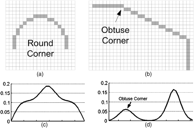
Thus, the image shows an example of determining the circular angle (round corner) (a) and the obtuse angle (obtuse corner) (b), which is not yet circular. For their determination, the curvature values are calculated, the graphs of which are shown in Figures (c) and (d).
The details of the algorithm are explained in [16].
Awrangjeb and Lu introduced a new CPDA detector (Chord-to-Point Distance Accumulation, 2008) [18].
On the one hand, a Gaussian with a large σ reduces noise, but affects localization, on the other, a Gaussian with a small σ is sensitive to noise. To solve these problems, Awrangjeb and Lu proposed a chord-to-point distance accumulation (CPDA) method using an adaptive threshold based on the ideas of Han and Poston. The CPDA method uses a discrete curvature estimate that is resistant to local variations. The authors use 3 chords of various lengths to estimate 3 normalized discrete values of curvature at each point of the smoothed curve. [19]
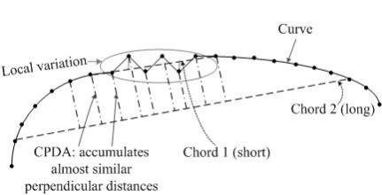
Since the detector uses a larger neighborhood, it is less sensitive to noise and local variations on the curve. The CPDA detector is a further development of the CSS detector. Steps:
You may notice that modern algorithms have become more complex. However, Harris and FAST detectors are the most frequently used and computationally fast algorithms for determining angles.
The article does not consider such detectors as Harris-Laplace, Hessian-Laplace, DoG, LoG, Harris-Affine, Hessian-Affine, Salient Regions, because although they allow you to determine angles, they should be more attributed to blobs detectors (drops blob) [five]
Also, this article does not exhaust the entire set of angle determination algorithms, due to their large number and specificity of application to subject areas. Some of the algorithms are more of theoretical interest than practical. The article describes the main algorithms for determining the angles that are most often found in the literature.
For example, there are also the following algorithms (with articles):
It is worth noting that this is not the whole list.
Below is a comparative table of angle detectors taken from [2].
Comparison of angle detectors (1 - Very bad, 2 - bad, 3 - satisfactory, 4 - good, 5 - excellent).
The behavior of corner detectors on the artificial test pattern of Smith.
The behavior of corner detectors on the test image of the house (House Test Image).
PS: I tried to review the main angle detectors. I hope that I did it. If the article has inaccuracies, please send messages to the PM. And, maybe, some algorithms are written too generalized, but if I wrote all the details, then the article would have grown to even larger sizes, if I had lost the thread of the story.
[1] Konushin A. Point feature tracking. Computer graphics and multimedia. Issue number 1 (5) / 2003 .
[2] Abhishak Yadav, Poonam Yadav. Digital Image Processing, 2009.
[3] Accurate Junction Detection and Characterization in Natural .
[4] An overview of characteristic point detection methods .
[5] Tinne Tuytelaars, Krystian Mikolajczyk. Local Invariant Feature Detectors: A Survey, 2008.
[6] Harris Corner Detector .
[7] http://www.cs.toronto.edu/~jepson/csc420/notes/imageFeaturesIIBinder.pdf .
[8] MH Miroslav Trajkovii. Fast corner detection, 1998.
[9] T. Shi. Good Features to Track, 1994.
[10] V. Rodehorst, A. Koschan. Comparison and evaluation of feature point detectors, 2006.
[11] Lecture 13. Interest Point Detection, 2004 .
[12] B. Smith. SUSAN - A new approach to low level, 1997.
[13] ER a. T. Drummond. Fusing Points and Lines for High Performance Tracking, 2005.
[14] RP a. TD Edward Rosten. Faster and better: a machine learning approach to corner detection, 2008.
[15] A. Rattarangsi, WUMWU Dept. of Electr. & Comput. Eng. and Analysis, Machine Analysis, IEEE Transactions on (Volume: 14, Issue: 4), 1992.
[16]X. Chen He, N. Yung. Corner detector based on global and local curvature, 2008 .
[17] RS Farzin Mokhtarian. Robust Image Corner Detection Through Curvature Scale Space, 1998.
[18] M. Awrangjeb. CPDA, 2009 .
[19] SMM Kahaki, 2014 Contour-Based Corner Detection and Classification.
[20] COMPSCI 773 feature point detection .
[21] Andres Solis Montero, Milos Stojmenović, Amiya Nayak. Robust Detection of Corners and Corner-line links in images. 10th IEEE International Conference on Computer and Information Technology (CIT 2010), 2010.
[22] SC Bae, IS Kweon and CD Yoo. COP: a new corner detector. Pattern Recogn. Lett., 2002.
- Introduction
- Properties of special points
- Angle detectors
- Moravec
- Harris
- Shi-tomasi
- Furstner
- Susan
- Trajkovic
- FAST
- CSS
- Detector based on global and local curvature properties
- CPDA
- findings
Introduction
')
In order to extract some interpreted information from an image, it is necessary to bind to local features of the image. On the image it is possible to highlight particular points A particular point m , or point feature (key point), an image is an image point whose neighborhood o (m) can be distinguished from the neighborhood of any other point of the image o (n) in some other neighborhood of the singular point o 2 (m) . For the majority of algorithms, a rectangular window measuring 5x5 pixels is taken as the neighborhood of the image point. The process of determining the singular points is achieved by using a detector and a descriptor.
A detector is a method of extracting specific points from an image. The detector ensures the invariance of finding the same singular points with respect to image transformations.
Descriptor is an identifier of a singular point that distinguishes it from the rest of the set of singular points. In turn, descriptors should ensure the invariance of finding a correspondence between specific points with respect to image transformations [1].
Properties of special points
In 1992, Haralick and Shapir [10] identified the following requirements for particular points as the following properties:
- Distinctness - a particular point should clearly stand out from the background and be distinguishable (unique) in its neighborhood.
- Invariance - the definition of a singular point must be independent of affine transformations.
- Stability (stability) - the definition of a particular point should be resistant to noise and errors.
- Uniqueness — besides local distinctness, the singular point must have global uniqueness to improve the distinctiveness of repeating patterns.
- Interpretability (interpretability) - special points should be determined so that they can be used to analyze matches and identify interpretable information from an image.
Interestingly, in [5], Tuytelaars and Mikolajczyk (2006) identified the following properties that particular points should have:
- Repeatability (repeatability) - a particular point is in the same place of the scene or image object, despite the changes in the point of view and illumination.
- Distinctiveness / informativeness (distinctiveness / informativeness) - the neighborhoods of singular points must be very different from each other, so that it is possible to identify and match particular points.
- Locality — A particular point must occupy a small area of the image in order to reduce the probability of sensitivity to geometric and photometric distortions between two images taken at different points of view.
- Quantity (quantity) - the number of detected points should be large enough so that they are enough to detect even small objects. However, the optimal number of singular points depends on the subject area. Ideally, the number of detected points should be adaptively determined using a simple and intuitive threshold. The density of the location of special points should reflect the information content of the image to ensure its compact representation.
- Accuracy (accuracy) - the detected special points must be precisely localized, both in the original image and taken on a different scale.
- Efficiency (efficiency) - the time of detection of specific points on the image should be valid in time-critical applications.
In general, these properties intersect with [10], but are interpreted differently.
Angle detectors
There are many algorithms for determining the special points, designed for different applications. In this article, I pay attention to angle detectors (or how they are called corner detector).
Angles (corners) are particular points that are formed from two or more faces, and faces usually define the boundary between different objects and / or parts of the same object. [2] In another way, we can say that the angles are the point at which in the neighborhood the intensity varies relative to the center (x, y) . Angles are determined by coordinates and changes in the brightness of the surrounding points of the image. The main property of such points is that in the area around the corner of the image gradient two dominant directions prevail, which makes them distinguishable. Gradient is a vector quantity that indicates the direction of the steepest increasing of the image intensity function I (x, y) . Since the image is discrete, the gradient vector is determined through the partial derivatives along the x and y axes through changes in the intensities of the adjacent image points. Most methods consider angularity depending on a derivative of the 2nd order, therefore, in general, methods are sensitive to noise.
Depending on the number of intersected faces, there are different types of angles: L-, Y- (or T-), and X- connected [3] (some still have swept-connected angles [2]). Different corner detectors react differently to each of these types of corners.
Approaches to the definition of singular points can be divided into 3 categories [10]:
- Based on image intensity: feature points are calculated directly from image pixel intensity values.
- Using contours of the image: the methods extract contours and look for places with the maximum curvature value or make a polygonal approximation of the contours and determine the intersection. These methods are sensitive to the vicinity of the intersections, as the extraction can often be wrong in places where 3 or more edges intersect.
- Based on the use of the model: models with intensity are used as parameters that adapt to the template images to sub-pixel accuracy. Have limited use with special points of special types (for example, L-connected angles), depend on the patterns used.
In practice, methods based on image intensity are the most common for widespread use.
Next, I will consider descriptions of the main detectors of singular points defining angles. Then a comparative table of detectors will be presented with conclusions about their applicability to various situations and, finally, images with corner detectors applied to them.
Moravec
Work in the study of image binding using singular points began the Moravec detector (Moravec, 1977). The Moravec detector is the simplest of all. The author considers the change in the brightness of a square window W (usually 3x3, 5x5, 7x7 pixels) relative to the point of interest when the window W is shifted by 1 pixel in 8 directions (horizontal, vertical and diagonal) [4]. Algorithm:
- For each pixel (x, y) in the image, calculate the change in intensity

- Build a map of the probability of finding the angles in each pixel (x, y) of the image by calculating the evaluation function
 . That is, the direction that corresponds to the smallest change in intensity is determined, since the corner must have adjacent edges.
 - Trim pixels in which C (x, y) values are below threshold T.
- Remove duplicate corners by applying the local maxima of the response function (non-maximal suppression). All obtained non-zero map elements correspond to the angles in the image.
Moravec detector has anisotropy property in 8 directions of window displacement. The main disadvantages of the detector under consideration are the lack of rotation transformation invariance and the occurrence of detection errors in the presence of a large number of diagonal edges [2].
Harris
Studies have shown that the most optimal detector of L-connected angles is the well-known Harris detector (also called the Plessey operator, the Harris and Stephens detector, Plessey operator, Harris and Stephens detector, 1988) [5] [6].
Harris and Stephens improved the Moravec detector by introducing anisotropy in all directions, i.e. consider the derivatives of the brightness of the image to study changes in brightness in many directions. They introduce derivatives in some principal directions.
For this image I, consider the window W (usually the window size is 5x5 pixels, but may depend on the image size) in the center (x, y) , as well as its shift by (u, v) .
Then the weighted sum of squared differences (sum of squared differences (SSD)) between the shifted and initial window (i.e., the change in the neighborhood of the point (x, y) when shifted by (u, v) ) is equal to:
where w (x, y) is a weight function (usually a Gaussian function or a binary window is used).
M - autocorrelation matrix:
The angle is characterized by large changes in the function E (x, y) in all possible directions (x, y) , which is equivalent to the eigenvalues of matrix M that are large in modulus. The location of the eigenvalues is shown in the following figure.
Since it is a laborious task to directly consider eigenvalues, Harris and Stephen proposed a measure of response [7]:
where k is an empirical constant,
.Thus, the value of R is positive for angular singular points. Then the points are cut off by the found threshold R (i.e., those points for which the value of R is less than a certain threshold are excluded from consideration). Next are the local maxima of the response function (non-maximal suppression) over a neighborhood of a given radius and are selected as corner singular points.
The Harris detector is invariant to rotations, partially invariant to affine changes in intensity. The disadvantages include the sensitivity to noise and the dependence of the detector on the scale of the image (to eliminate this drawback, Harris's multi-scale detector is used).
Shi-tomasi
The Shih-Tomasi angular detector (Shi-Tomasi or Kanade-Tomasi, 1993) largely coincides with the Harris detector, but differs in the calculation of the response measure: the algorithm directly calculates the value
since the assumption is made that the search for angles will be more stable. The authors use the same equation to analyze the optical flux of Lucas and Canada (Lucas and Kanade). The details of the algorithm are given in [8] and [9].Furstner
Förstner and Gölch (Förstner and Gülch, 1987) were the first to describe a method that uses the same angularity measure as the Harris detector. They used a more complex computational implementation [8]. Unlike the Harris detector, the eigenvalues are computed explicitly. The response function of the Förstner angle is defined as follows:
Also for the correctness of the definition is considered a measure of the roundness of the angle, equal to:
.In practice, the Förstner detector is often used to extend the capabilities of the Harris detector — to find circular singular points along with the corners. Also, the algorithm has the best localization property [2].
A more detailed description of the algorithm is presented in Wikipedia , as well as in [10], [11].
Susan
The SUSAN (Smallest Univalue Segment Assimilation Nucleus) algorithm was proposed by Smith and Brady (Smith and Brady, 1997) [5].
Angles are determined by segmentation of circular neighborhoods into similar (orange) and unlike (blue) areas. Angles are located where the relative area of similar areas (similar USAN) reaches a local minimum below a certain threshold.
For each pixel, a circular area of fixed radius is considered. The center of the pixel is called the core, its intensity value is remembered. All other pixels are divided into 2 categories: similar (orange) and unlike (blue) areas, depending on whether the intensity of the core is similar or not. Where there is a section of the image under a circular area unchanged, similar areas occupy almost the entire area, on the edges this ratio drops to 50%, at the corners it decreases to about 25%. Thus, the angles are located where the relative area of similar areas (similar USAN) reaches a local minimum below a certain threshold. To increase the stability of the algorithm, the authors assign higher weights to the pixels closest to the core. The steps of the algorithm are as follows:
- Place the center of the circular mask in the core.
- Inside the circular mask, calculate the number of pixels that have similar intensity with the core using the following formula (the found pixels determine the USAN):

 - a point inside the mask;
 - core center;
 - point intensity ;
t is the difference threshold of intensities; - the result of the comparison.
 - Subtract the USAN size from the geometric threshold to obtain an image with angles, using the following formula:
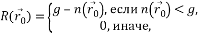
 - the initial value of the edge response. SUSAN principle: the smaller the USAN area, the greater the edge response.
g is the geometric threshold. - number of pixels in USAN, i.e. USAN area.
 - Find the centroids of the USAN areas and their proximity to each other and identify false positives.
- Select specific points by searching for local maxima of the response function (nonmaximum suppression).
The algorithm shows good accuracy for all kinds of angles, but is not susceptible to blurring on images. Details are given in [12].
Trajkovic
Tryakovits and Hedley (Miroslav Trajkovic and Mark Hedley, 1998) in the article “Fast corner detection” introduced a new type of detector - the operator Tryakovits [8]. Initially, the authors made demands on him to become the most popular angle detector and have the minimum computational cost. First, the 4-neighbor algorithm Trajkovic4 was developed.
The detector checks the area around the pixel by examining nearby pixels: let c be the pixel to be considered, and P be the point on the circle S N at the center at the point N. Point P ' is the point opposite to P in diameter.
Response functions (authors call it CRN, Corner Request Function) are defined as:
where N is the center point;
P and P ' are two points opposite in diameter around point N ;
S N - sampled circle on an image with a radius of 3, 5, 7 pixels.
The CRN value will be large when there is no direction in which the central pixel resembles two nearby pixels in diameter. Since the calculation in any direction gives an upper limit of min, the horizontal and vertical directions are checked first to determine whether it makes sense to move on to the full calculation of R N.
In comparison with the Harris detector, the frequency of repeatability of the Trajkovic4 algorithm is worse, but localization is comparable with the definition of L-connected angles and is superior to other types of angles.
Also, the disadvantages include the fact that this 4-neighbor operator falsely reacts to diagonal edges and is sensitive to noise [2]. Therefore, use the 8-connected version of this algorithm Trajkovic8. Trajkovic8 differs from Trajkovic4 in the way it calculates angularity. However, Trajkovic8 still finds false angles on some diagonal edges of the object (it does not show itself well on artificial images). Detailed descriptions of the algorithms are given in [2] and [8].
FAST
Rosten and Drummond (Edward Rosten and Tom Drummond, 2005) introduced a rather successful FAST algorithm (Features from Accelerated Segment Test) - features of the accelerated segment tests.
The algorithm considers a circle of 16 pixels (drawn by the Bresenham algorithm) around candidate point P. A point is angular if for the current considered point P there are N adjacent pixels on a circle whose intensities are greater than I P + t or the intensities of all are less than I P -t , where I P is the intensity of point P , t is a threshold value. Next, you need to compare the intensity at the vertical and horizontal points on the circle numbered 1, 5, 9 and 13 with the intensity at point P (in order to cut off the false candidates as quickly as possible). If the condition I Pi > I P + t or I Pi <I P + t, i = 1, .., 4 , is fulfilled for 3 of these points, then a complete test is performed for all 16 points [13]. Experiments have shown that the smallest value of N , at which singular points begin to be detected steadily, is N = 9 .
Initially, the original algorithm was FAST-12 . There are modifications of the algorithm: tree-like FAST-9 and FAST-12 (the tree based FAST-9 and FAST-12).
The original algorithm has several drawbacks, for example, several particular points can be found near a certain neighborhood, the efficiency of the algorithm depends on the order of image processing and the distribution of pixels.
In [14], the authors Edward Rosten, Reid Porter, and Tom Drummond (2008) introduce improvements to the FAST algorithm, namely, that they use machine learning to determine specific points.
This algorithm they called FAST-ER (ER - Enhanced Repeatability, improved repeatability). The algorithm is stable to the property of repeatability: on the same scene, viewed from different angles, there are special points belonging to the same objects.
This algorithm uses a ring of a circle of more than 1 pixel, rather than in FAST (48 pixels). The authors use the ID3 algorithm to classify special points (whether the candidate point is special) using decision trees. The ID3 algorithm optimizes the order in which pixels are processed, resulting in the most computationally efficient detector.
The cost function of the decision tree is calculated as follows:
R is a measure of repeatability;
N is the number of detected singular points;
S is the number of nodes in the decision tree.
Details are described in [14].
FAST-ER is better than FAST, but slower in execution speed. The authors concluded that the FAST-ER detector is the best in relation to the repeatability property.
CSS
Rattarangsi and Chin (1992) [15] proposed an algorithm based on curvature scale space (CSS) that detects angles on flat curves. CSS is suitable for extracting invariant geometric features on a flat curve at various scales.
The algorithm determines singular points using several scales of the same image. However, it is computationally complex and detects false angles in circular areas. [sixteen]
Farzin Mokhtarian and Riku Suomela (1998) [17] improved the algorithm in noise resistance. This algorithm applies to a black and white image and includes the following steps:
- Apply the Canny Boundary Detector (Canny) to the image and get a binary boundary map.
- Select border outlines from a binary map. Check the ends of the contours for adjacency with others, if this is the case, then re-fill the boundary before connecting. Mark this point as a T-connected angle if the end of the contour is connected to the border.
- Calculate the curvature values of each contour on the largest σ high scale. The initial values are the local maximums of curvature, provided that the value of the curvature is higher than the threshold t and twice as large as the neighboring local minima.
- Sort angles in descending order from the largest to the smallest scale in order to improve the localization property.
- Compare T-connected corners with the other corners and, if they are close to each other, remove one of the corners.
The image shows 2 cases of face spacing: the T-connected gap is marked as an angle (T-corner point), and the gap between the ends of the contours (gap) is filled.
This algorithm has the following disadvantages: the image at only one scale is used to determine the number of angles (step 3), and the images at several scales for localization. As a result, the algorithm skips angles when σ is large, and detects false ones, when σ is small. [sixteen]
A number of improvements were made to the algorithm: in 2001 F. Mokhtarian and R. Suomela in the article “Robust image corner detection through curvature scale space” (suggested improved CSS) and in 2008 - He and Yung in the article “Corner detector on global and local curvature properties ”, as well as the CPDA detector.
Detector based on global and local curvature properties
He and Yung (2008) in the article “Corner detector based on global and local curvature properties” offer an improvement to the CSS algorithm. They claim that traditional computational algorithms consider local properties of the image, often falsely determining the noise at specific points or missing small details of an object. This algorithm balances the global and local properties of the curvature level of the faces to extract the corners.
As a result, He and Yung offer the following solution:
- Detect boundaries, for example, with a Canny Canny detector to get a binary boundary map.
- Select contours as in the CSS algorithm.
- Calculate the curvature values for a fixed small scale (so as not to miss the true angles), consider the local maxima of the absolute values of curvature, which are noted as potential corner candidates.
- Calculate the threshold, based on the average value of the curvature in the considered area. Remove circular angles by comparing the curvature values of the corner candidates with an adaptive threshold.
- Calculate the angle values of the remaining corner candidates using the adaptive considered area and remove the false candidates.
- Consider the ends of open contours and mark them as corners if they are not close to each other.
Thus, the image shows an example of determining the circular angle (round corner) (a) and the obtuse angle (obtuse corner) (b), which is not yet circular. For their determination, the curvature values are calculated, the graphs of which are shown in Figures (c) and (d).
The details of the algorithm are explained in [16].
CPDA
Awrangjeb and Lu introduced a new CPDA detector (Chord-to-Point Distance Accumulation, 2008) [18].
On the one hand, a Gaussian with a large σ reduces noise, but affects localization, on the other, a Gaussian with a small σ is sensitive to noise. To solve these problems, Awrangjeb and Lu proposed a chord-to-point distance accumulation (CPDA) method using an adaptive threshold based on the ideas of Han and Poston. The CPDA method uses a discrete curvature estimate that is resistant to local variations. The authors use 3 chords of various lengths to estimate 3 normalized discrete values of curvature at each point of the smoothed curve. [19]
Since the detector uses a larger neighborhood, it is less sensitive to noise and local variations on the curve. The CPDA detector is a further development of the CSS detector. Steps:
- Find borders on the image using the Canny Boundary Detector.
- .
- , , .
- T- T- .
- .
- , , .
- 3 , 3 .
- 3 .
- «» .
- .
- Find the angles between the ends of the smoothed loops (if any) and the detected angles, if they are sufficiently distant from them.
- Each of the T-connected corners found add to the detected corners if it is sufficiently removed from them. [18]
findings
You may notice that modern algorithms have become more complex. However, Harris and FAST detectors are the most frequently used and computationally fast algorithms for determining angles.
The article does not consider such detectors as Harris-Laplace, Hessian-Laplace, DoG, LoG, Harris-Affine, Hessian-Affine, Salient Regions, because although they allow you to determine angles, they should be more attributed to blobs detectors (drops blob) [five]
Also, this article does not exhaust the entire set of angle determination algorithms, due to their large number and specificity of application to subject areas. Some of the algorithms are more of theoretical interest than practical. The article describes the main algorithms for determining the angles that are most often found in the literature.
For example, there are also the following algorithms (with articles):
- Rotary invariant operator DET (probably one of the first detectors). PR Beaudet. Rotationally invariant image operators. In Proc. IAPR1978, pages 579–583, 1978.
- Kitchen-Rosenfeld detector. L. Kitchen and A. Rosenfeld. Gray Level Corner Detection. Pattern Recognition Letters, pp. 95-102, 1982.
- Detector Wang-Brady. H. Wang and M. Brady. Real-time corner detection algorithm for motion estimation. Image and Vision Computing, vol. 13: 9, pp. 695-703, 1995.
- SCD detector (Structure-based corner detector). Fei Shen, Han Wang. Real Time Gray Level Corner Detector. 2000
- COP detector (Crosses as Oriented Pair). SC Bae, IS Kweon and CD Yoo. COP: a new corner detector. Pattern Recogn. Lett. 2002
- Improved detector based on Harris-Stephen and Shi-Tomasi detectors. Lidia Forlenza, Patrick Carton, Domenico Accardo, Giancarmine Fasano and Antonio Moccia. Real Time Corner Detection for Miniaturized Electro-Optical Sensors Onboard Small Unmanned Aerial Systems. 2012
- Zhang Detector. Jun Zhang, Tingjin Luo, Gui Gao, and Lin Lian. Junction Point Detection Algorithm for SAR Image, 2013.
It is worth noting that this is not the whole list.
Comment
, . , , . , , ( ) 2 .
 [16]
[16] 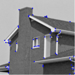 [2]
[2]
[16] [2]Below is a comparative table of angle detectors taken from [2].
Comparison of angle detectors (1 - Very bad, 2 - bad, 3 - satisfactory, 4 - good, 5 - excellent).
| Operator (algorithm) | Detection efficiency | Localization | Frequency of occurrence | Noise resistance | Speed |
|---|---|---|---|---|---|
| Beaudet | 3 | 3 | 4 for affine transformations, 2 for scaling | 2 | four |
| Moravec | 3 | four | 3 | 3 | four |
| Kitchen & Rosenfeld | 3 | 3 | 3 | 3 | 3 |
| Furstner | four | four | 5 for affine transformations, 3 for scaling | four | 2 |
| Plessey | four | 4 for L-connected angles, 2 for other types | 5 for affine transformations if an anisotropic gradient is calculated, 3 for scaling | 3 | 2 |
| Deriche | 3 (?) | four | four | 2 | four |
| Wang & brady | four | four | four | 3 | four |
| Susan | four | 1 for blurry images, 4+ otherwise | 4 for scaling, 2 for affine transformations | five | four |
| CSS | four | four | five | four | Depends strongly on the border detector used |
| Trajkovic & Hedley (4-neighbors) | 2 | four | 3 (not invariant to rotations) | 2 | five |
| Trajkovic & Hedley (8-neighbors) | 3 | four | 3+ (not invariant to turns) | four | five |
| Zheng & wang | four | 4 for L-connected angles, 3 for other types | 5 for affine transformations, 3 for scaling | 3 | 3 |
The behavior of corner detectors on the artificial test pattern of Smith.
| Operator (algorithm) | Work result |
|---|---|
| Moravec [2] |  |
| Plessey | 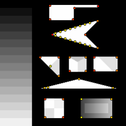 |
| Susan | 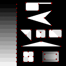 |
| Förstner [10] |  |
| Trajkovic4 | 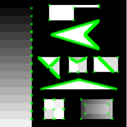 |
| Trajkovic8 | 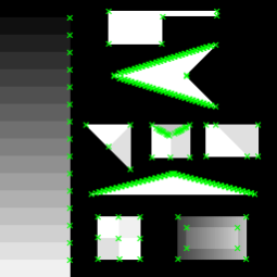 |
| Shi-Tomasi [20] | 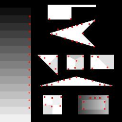 |
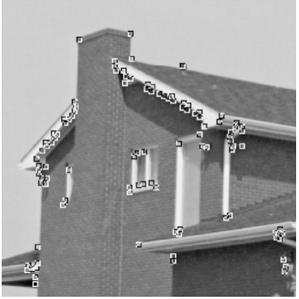
The behavior of corner detectors on the test image of the house (House Test Image).
| Operator (algorithm) | Work result |
|---|---|
| Moravec | 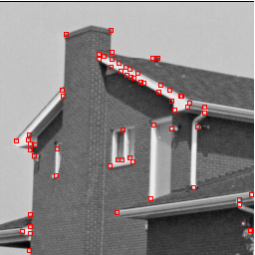 |
| Plessey |  |
| SUSAN [16] |  |
| Furstner | 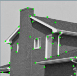 |
| FAST [21] |  |
| Original CSS [16] |  |
| Enhanced CSS [16] | 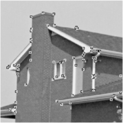 |
| Corner detector based on global and local properties 2008 [16] |  |
| Kitchen-Rosenfeld [22] | 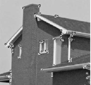 |
| COP [22] | 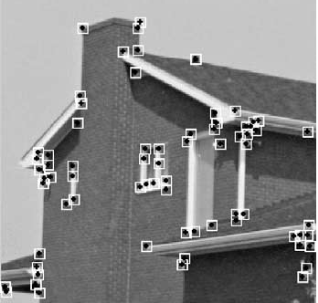 |
PS: I tried to review the main angle detectors. I hope that I did it. If the article has inaccuracies, please send messages to the PM. And, maybe, some algorithms are written too generalized, but if I wrote all the details, then the article would have grown to even larger sizes, if I had lost the thread of the story.
Bibliography
[1] Konushin A. Point feature tracking. Computer graphics and multimedia. Issue number 1 (5) / 2003 .
[2] Abhishak Yadav, Poonam Yadav. Digital Image Processing, 2009.
[3] Accurate Junction Detection and Characterization in Natural .
[4] An overview of characteristic point detection methods .
[5] Tinne Tuytelaars, Krystian Mikolajczyk. Local Invariant Feature Detectors: A Survey, 2008.
[6] Harris Corner Detector .
[7] http://www.cs.toronto.edu/~jepson/csc420/notes/imageFeaturesIIBinder.pdf .
[8] MH Miroslav Trajkovii. Fast corner detection, 1998.
[9] T. Shi. Good Features to Track, 1994.
[10] V. Rodehorst, A. Koschan. Comparison and evaluation of feature point detectors, 2006.
[11] Lecture 13. Interest Point Detection, 2004 .
[12] B. Smith. SUSAN - A new approach to low level, 1997.
[13] ER a. T. Drummond. Fusing Points and Lines for High Performance Tracking, 2005.
[14] RP a. TD Edward Rosten. Faster and better: a machine learning approach to corner detection, 2008.
[15] A. Rattarangsi, WUMWU Dept. of Electr. & Comput. Eng. and Analysis, Machine Analysis, IEEE Transactions on (Volume: 14, Issue: 4), 1992.
[16]X. Chen He, N. Yung. Corner detector based on global and local curvature, 2008 .
[17] RS Farzin Mokhtarian. Robust Image Corner Detection Through Curvature Scale Space, 1998.
[18] M. Awrangjeb. CPDA, 2009 .
[19] SMM Kahaki, 2014 Contour-Based Corner Detection and Classification.
[20] COMPSCI 773 feature point detection .
[21] Andres Solis Montero, Milos Stojmenović, Amiya Nayak. Robust Detection of Corners and Corner-line links in images. 10th IEEE International Conference on Computer and Information Technology (CIT 2010), 2010.
[22] SC Bae, IS Kweon and CD Yoo. COP: a new corner detector. Pattern Recogn. Lett., 2002.
Source: https://habr.com/ru/post/244541/
All Articles