Equalization of histograms for image enhancement
Hello. Now we are preparing a monograph with a supervisor for publication, where we are trying to tell in simple words about the basics of digital image processing. This article reveals a very simple, but at the same time very effective method of improving the quality of images - equalization of histograms.
For simplicity, we will begin consideration with monochrome images (ie, images containing information only about the brightness, but not about the color of the pixels). The image histogram will be called the discrete function H, defined on the set of values [0; 2 bpp ], where bpp is the number of bits allocated for coding the brightness of one pixel. Although it is not necessary, histograms are often normalized to the range [0; 1], dividing each value of the function H [i] by the total number of pixels of the image. Tab. 1 shows examples of test images and histograms based on them:
Tab. 1. Images and their histograms
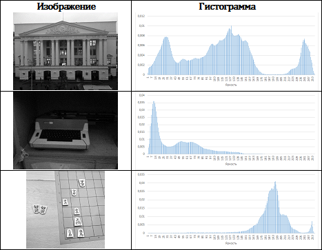
Having carefully studied the corresponding histogram, we can draw some conclusions about the original image itself. For example, histograms of very dark images are characterized by the fact that non-zero values of the histogram are concentrated near zero brightness levels, and for very bright images, on the contrary, all non-zero values are concentrated on the right side of the histogram.
Intuitively, it can be concluded that the most convenient person for perception will be an image whose histogram is close to a uniform distribution. Those. to improve the visual quality of the image, it is necessary to apply such a transformation so that the result histogram contains all possible brightness values and at the same time in approximately the same amount. This conversion is called histogram equalization and can be performed using the code in Listing 1.
Listing 1. Implementing a histogram equalization procedure
As a result of histogram equalization in most cases, the dynamic range of the image is significantly expanded, which allows you to display previously unnoticed details. This effect is particularly pronounced in dark images, as shown in Table. 2. In addition, it is worth noting another important feature of the equalization procedure: unlike most filters and gradation transformations that require setting parameters (apertures and gradation conversion constants), histogram equalization can be performed in fully automatic mode without operator intervention.
Tab. 2. Images and histograms after equalization
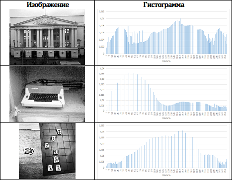
It is easy to see that histograms after equalization have peculiar noticeable gaps. This is due to the fact that the dynamic range of the output image is wider than the range of the original. Obviously, in this case, the mapping considered in Listing 1 cannot provide nonzero values in all histogram pockets. If you still need to achieve a more natural look of the output histogram, you can use a random distribution of the values of the i-th histogram pocket in some of its surroundings.
It is obvious that equalization of histograms makes it possible to easily improve the quality of monochrome images. Naturally you want to apply a similar mechanism to color images.
Most not very experienced developers present an image in the form of three RGB color channels and try to apply the histogram equalization procedure to each color one separately. In some rare cases, this allows you to succeed, but in most cases the result is so-so (the colors are unnatural and cold). This is due to the fact that the RGB model does not accurately display the color perception of a person.
Think of a different color space - HSI. This color model (and others related to it) is very widely used by illustrators and designers as they allow one to operate with the concepts of color tone, saturation and intensity that are more familiar to humans.
If we consider the projection of the RGB cube in the direction of the diagonal white-black, we get a hexagon, the corners of which correspond to primary and secondary colors, and all gray shades (lying on the diagonal of the cube) are projected into the center point of the hexagon (see Fig. 1):
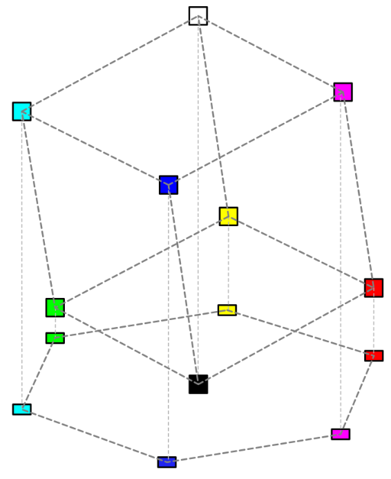
Fig. 1. Projection of the color cube
To use this model to encode all the colors available in the RGB model, you need to add a vertical axis of lightness (or intensity) (I). The result is a hex cone (Fig. 2, Fig. 3):
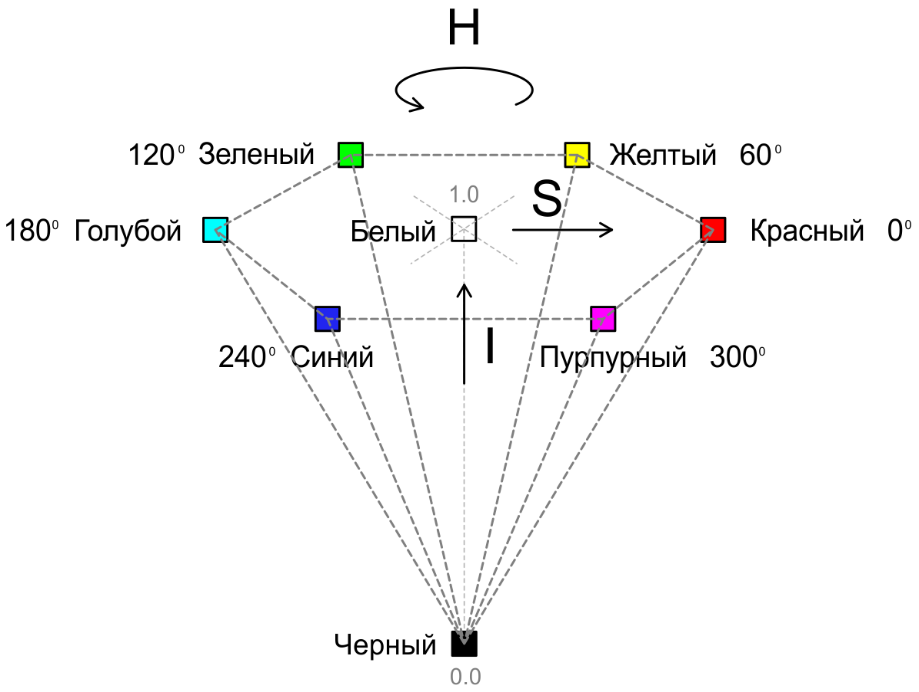
Fig. 2. HSI Pyramid (vertices)
In this model, the color tone (H) is set by the angle relative to the red axis, the saturation (S) represents the purity of the color (1 means a completely pure color, and 0 corresponds to a shade of gray). At zero saturation, the tone is meaningless and undefined.

Fig. 3. HSI Pyramid
Tab. Figure 3 shows the image decomposition in HSI components (white pixels in the tone channel correspond to zero saturation):
Tab. 3. HSI color space
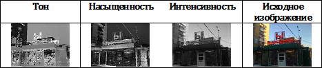
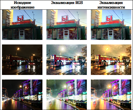
It is believed that to improve the quality of color images it is most effective to apply the procedure of equalization to the intensity channel. This is what is shown in Table. four
Tab. 4. Equalization of various color channels
I hope this material seemed at least as interesting to you as maximum useful. Thank.
For simplicity, we will begin consideration with monochrome images (ie, images containing information only about the brightness, but not about the color of the pixels). The image histogram will be called the discrete function H, defined on the set of values [0; 2 bpp ], where bpp is the number of bits allocated for coding the brightness of one pixel. Although it is not necessary, histograms are often normalized to the range [0; 1], dividing each value of the function H [i] by the total number of pixels of the image. Tab. 1 shows examples of test images and histograms based on them:
Tab. 1. Images and their histograms
Having carefully studied the corresponding histogram, we can draw some conclusions about the original image itself. For example, histograms of very dark images are characterized by the fact that non-zero values of the histogram are concentrated near zero brightness levels, and for very bright images, on the contrary, all non-zero values are concentrated on the right side of the histogram.
Intuitively, it can be concluded that the most convenient person for perception will be an image whose histogram is close to a uniform distribution. Those. to improve the visual quality of the image, it is necessary to apply such a transformation so that the result histogram contains all possible brightness values and at the same time in approximately the same amount. This conversion is called histogram equalization and can be performed using the code in Listing 1.
Listing 1. Implementing a histogram equalization procedure
- procedure TCGrayscaleImage . HistogramEqualization ;
- const
- k = 255 ;
- var
- h : array [ 0 .. k ] of double ;
- i , j : word ;
- begin
- for i : = 0 to k do
- h [ i ] : = 0 ;
- for i : = 0 to self . Height - 1 do
- for j : = 0 to self . Width - 1 do
- h [ round ( k * self . Pixels [ i , j ] ) ] : = h [ round ( k * self . Pixels [ i , j ] ) ] + 1 ;
- for i : = 0 to k do
- h [ i ] : = h [ i ] / ( self . Height * self . Width ) ;
- for i : = 1 to k do
- h [ i ] : = h [ i - 1 ] + h [ i ] ;
- for i : = 0 to self . Height - 1 do
- for j : = 0 to self . Width - 1 do
- self . Pixels [ i , j ] : = h [ round ( k * self . Pixels [ i , j ] ) ] ;
- end ;
As a result of histogram equalization in most cases, the dynamic range of the image is significantly expanded, which allows you to display previously unnoticed details. This effect is particularly pronounced in dark images, as shown in Table. 2. In addition, it is worth noting another important feature of the equalization procedure: unlike most filters and gradation transformations that require setting parameters (apertures and gradation conversion constants), histogram equalization can be performed in fully automatic mode without operator intervention.
Tab. 2. Images and histograms after equalization
It is easy to see that histograms after equalization have peculiar noticeable gaps. This is due to the fact that the dynamic range of the output image is wider than the range of the original. Obviously, in this case, the mapping considered in Listing 1 cannot provide nonzero values in all histogram pockets. If you still need to achieve a more natural look of the output histogram, you can use a random distribution of the values of the i-th histogram pocket in some of its surroundings.
It is obvious that equalization of histograms makes it possible to easily improve the quality of monochrome images. Naturally you want to apply a similar mechanism to color images.
Most not very experienced developers present an image in the form of three RGB color channels and try to apply the histogram equalization procedure to each color one separately. In some rare cases, this allows you to succeed, but in most cases the result is so-so (the colors are unnatural and cold). This is due to the fact that the RGB model does not accurately display the color perception of a person.
Think of a different color space - HSI. This color model (and others related to it) is very widely used by illustrators and designers as they allow one to operate with the concepts of color tone, saturation and intensity that are more familiar to humans.
If we consider the projection of the RGB cube in the direction of the diagonal white-black, we get a hexagon, the corners of which correspond to primary and secondary colors, and all gray shades (lying on the diagonal of the cube) are projected into the center point of the hexagon (see Fig. 1):
Fig. 1. Projection of the color cube
To use this model to encode all the colors available in the RGB model, you need to add a vertical axis of lightness (or intensity) (I). The result is a hex cone (Fig. 2, Fig. 3):
Fig. 2. HSI Pyramid (vertices)
In this model, the color tone (H) is set by the angle relative to the red axis, the saturation (S) represents the purity of the color (1 means a completely pure color, and 0 corresponds to a shade of gray). At zero saturation, the tone is meaningless and undefined.
Fig. 3. HSI Pyramid
Tab. Figure 3 shows the image decomposition in HSI components (white pixels in the tone channel correspond to zero saturation):
Tab. 3. HSI color space
It is believed that to improve the quality of color images it is most effective to apply the procedure of equalization to the intensity channel. This is what is shown in Table. four
Tab. 4. Equalization of various color channels
I hope this material seemed at least as interesting to you as maximum useful. Thank.
')
Source: https://habr.com/ru/post/244507/
All Articles