Modeling pandemics using the Wolfram Language (Mathematica 10) using the example of Ebola

Translation of Vitaly Kaurov's post (Vitaliy Kaurov) " Modeling a Pandemic like Ebola with the Wolfram Language ".

I express my gratitude for the help in translating Wolfram Mathematica to the members of the VKontakte Russian-speaking community : Eva Frumen, Kurban Magomedov , Gleb Mikhnovts , Andrei the Meek .

Download the translation in the form of a Mathematica document that contains all the code used in the article here (archive, ~ 100 MB).
')
Data is essential for an impartial look to the future, but data alone is not yet a forecast. Scientific models are needed to predict the development of pandemics, terrorist attacks, natural disasters, market crashes and other complex phenomena of our world. One of the tools to combat the current terrifying outbreak of Ebola is the creation of a computer model of the possible spread of the virus. Understanding where and how quickly an outbreak can manifest itself, government agencies will be able to organize effective preventive measures to reduce the speed of transmission and, ultimately, stop the epidemic. Our goal now is to demonstrate the construction of a mathematical model that describes the global distribution of a pandemic based on real data. The model is applicable to any epidemic, but we will sometimes mention and use data on the current outbreak of Ebola as an example. The results should not be viewed as a realistic quantitative assessment of the current Ebola pandemic.



To show us all the science of computing pandemics, I asked Dr. Marco Thiel , who has already posted a description of various Ebola distribution models on the Wolfram Community forum (where readers can take part in the discussion). We worked together on the software implementation of the global pandemic spread model below. This task has become much simpler, thanks to new tools added recently to the Wolfram Language programming language ( Mathematica 10). Marco is an applied mathematician specializing in theoretical physics and dynamical systems. His research work was covered at BBC News and, thanks to its applied mathematical nature, it covers very different areas: from the stability of the solar system to the mating patterns of fireflies, forensic mathematics and many other areas. Working with such a wide range of real-world tasks, Marco, his colleagues and students from the University of Aberdeen have made Wolfram technologies a part of their life. For example, the main part of the program for this blog is written by India Bruckner (India Bruckner), a very talented schoolgirl from the Aberdeen school of St.. Margarita for girls, with whom Marco worked on the summer project.

According to The New York Times , the current outbreak of Ebola fever was "the most ruthless, eclipsed the outbreak of 1976, when the virus was detected." According to data from October 27, 2014, at least 18 people have received or are receiving treatment in Europe and America, mostly health workers and humanitarian workers who have caught the Ebola virus in West Africa and returned home for treatment. According to a report by the US Centers for Disease Control and Prevention (CDC), released in September, in the worst case, the number of Ebola cases will exceed a million in four months. Medicines or vaccines against the virus approved by the Food and Drug Administration (FDA) do not yet exist, leading to death in 60-90% of cases and spread of the disease through contact with various physiological fluids of infected people. The following shows what the situation looks like in the outbreak of a pandemic in West Africa now according to The New York Times .

In [2]: =



Out [2] =



Vitali: Marco, do you think mathematical modeling can help stop a pandemic?

Marco: The recent outbreak of the Ebola virus disease (EVD) shows how quickly diseases can be transmitted between people. The threat, of course, is not limited to BVVE. There are a large number of pathogens, such as various types of flu (H5N1, H7N9, etc.), which can cause a pandemic. In view of this, mathematical modeling of the ways of transmission (diseases) becomes even more significant. The authorities from medicine must make decisions on how to counter the threat. There are a large number of scientific articles on this topic, such as the recent publication of Dirk Brockmann in Science available here . Professor Brockmann also made several videos to illustrate the research. The video is available on YouTube ( part 1 , part 2 , part 3 ). It would be interesting to repeat some of the results from this article and generally investigate the issue using Mathematica .

Vitali: How to build a model that describes the spread of the disease?

Marco: Detailed models, such as GLEAMviz, are available online, and can be used by anyone interested in a problem. The model, like the others similar to it, has 3 levels: (1) an epidemic model describing the transmission of the disease in a hypothetical homogeneous population; (2) population data, such as population distribution and density; (3) the level describing the migration of the population. I used a similar model, relying on Mathematica's powerful algorithms: embedded databases and extensive data import capabilities. In addition, Mathematica's visualization algorithms allow the development of a new model for the spread of diseases. The advantages of self-modeling are full control over the program and its change in accordance with our requirements. The supervised Wolfram data available in Mathematica is a very convenient starting point for modeling and can be supplemented with data imported from external sources. This is one of the incarnations of Conrad Wolfram’s ideas about the general availability of computed data . Using the current Mathematica tools , we will be able to imagine the opportunities that will open up to us after all state / public data becomes computable.

There are various types of epidemiological models. Further, we mainly will use the so-called SIR-model (from the English. Susceptible Infected Recovered). The population is modeled by three types of individuals (three “boxes”): healthy individuals at risk or susceptible individuals (Susceptible) who can catch the disease through contact with those already infected (Infected); recovered and ceased to spread the disease of individuals (Recovered).



To simulate a flash using the Wolfram Language, we need equations that describe the number of people in each of these categories as a function of time. We will first use equations with discrete time. Assuming that there are only three categories of individuals that do not interact with each other, we can write the following:

In [3]: =



These equations mean that the number (in percentage terms) of susceptible / infected / recovered (Susceptibles / Infected / Recovered) at time t + 1 is equal to the same number at time t . Suppose that accidental contact of an infected individual with a susceptible leads to a new infection with probability b ; the probability of contact is proportional to the number of susceptible individuals (Sus), as well as the number of already infected (Inf). This assumption means that people leave the “box” of the susceptible and go into the “box” (category) of the infected.

In [6]: =



Further, we assume that people recover with probability c ; recovery is proportional to the number of sick people; so, the more cases, the more recovered.

In [9]: =



We will also need initial data on the number (in percent) of people in each of the categories. Note that the terms on the right side of the system, which characterize the interaction between the categories, always give a total of zero, so the total population size does not change. If we take the initial values ​​so that their sum is equal to one, then the population size will always be equal to one. This is an important distinctive feature of the model. Each person must be assigned to one of three "boxes"; we will carefully monitor the preservation of this property for the SIR model on the graphs, which we describe below! At the same time, there is a certain freedom in the interpretation of these three "boxes". So, in our last example, we will take into account the lethal outcomes. It seems logical to assume that the dead "leave" our population. To keep the population size constant, which is important in our view, we use a simple technique: we will consider the last group of recovered (Rec), as a multitude containing people who have really suffered from the disease and those who have died. It is quite reasonable to assume that neither the dead nor those who have recovered will be able to infect the rest of the population, i.e. they are inert to our model. Our simple assumption will be that a certain fixed percentage of people from the Rec group have suffered a disease (survived), while the rest will be considered dead. Thus, we include the dead in our model, so that they do not leave the group, and we do not consider the birth of new people. This ensures that the size of the population remains constant.

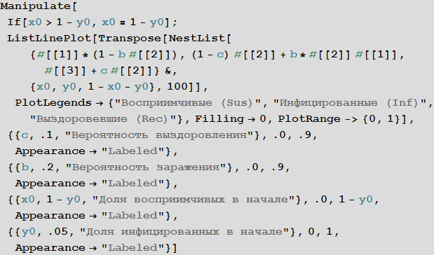
Here is the simplest implementation of the SIR model, allowing you to change the parameters:

In [12]: =



Out [12] =



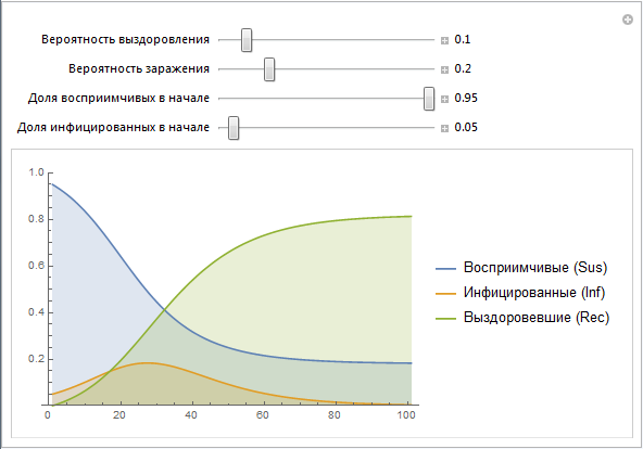
We use the vectors of values ​​Sus, Inf, Rec, which are constructed recursively. Later we will create a simpler implementation of this construct. Note that the parameters b and c contain a lot of effects that are not directly modeled at this stage. For example, the probability of infection b really describes the risk of infection, but at the same time it depends on the behavior of people (a large number of public events, public places, etc., can lead to an increase in the probability of infection, as it often happens, say, in educational institutions) , population density (high population density can lead to a greater likelihood of infection). The probability of recovery c depends on such things as: the quality of health care, the availability of doctors and so on. Later we will try to simulate some of the above factors.

Although the SIR model is probably not the most appropriate for describing an Ebola outbreak, this model is nevertheless not so far from the truth. People become infected through physical contact; the category of recovered can be considered from the percentage of surviving and deceased people, if we assume that reinfection is unlikely. In different countries and under different circumstances, the proportion of recovered / deceased varies greatly - we will model some of this later.

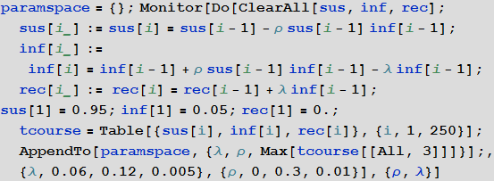
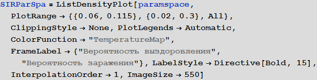
A more systematic way to study the SIR model is to study the so-called model parameter space. Depending on the parameters, we can visualize many different characteristics, for example, the largest number of cases, the total number of cases during an outbreak of infection from a virus. The axis of the diagram below shows the probabilities of infection and recovery, and the color on the diagram characterizes the percentage of infected people.

In [13]: =



In [14]: =



Out [14] =



The diagram clearly shows that with small values ​​of the probability of recovery and large values ​​of the probability of infection, more than 90% of people are sick, while in the opposite situation, about 5% of people are infected, which corresponds to their initial number.

Vitaliy: To move from pure mathematics to the modeling of processes occurring in the real world, we need data, let's say about human populations and their geographical location. How can we get this data?

Marco: We will combine several different sub-populations together (for example, airport, city, country, etc.) and study the spread of the disease between them. Each of these subpopulations can be modeled as a SIR model. When we begin to combine subpopulations, their individual dimensions will play a key role. Population data, like many other types of data, is embedded directly into Mathematica , which makes it quite easy to use them in our model.

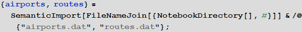
We will use the embedded data to improve the quality of our model and bring it to a logical conclusion, but at the beginning we can use the international airport network to simulate the transmission of the disease. For this we need a list of all airports and airways. At openflights.org you can find all the necessary information. I saved it to the airports.dat and routes.dat files.

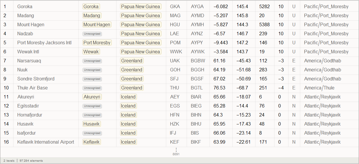
Vitaliy: We could use the functionality of semantic data import for working with external data. The SemanticImport function can import a file semantically, providing a Dataset object on output. Dataset and Association are new features that enable the creation of structured databases in Mathematica . A dataset can be not only rectangular multidimensional data arrays, but also arbitrary trees corresponding to data with an arbitrary hierarchy. Dataset makes it very easy to access and process any data in the database, so we will actively use it. A small part of the data contained in the airports.dat file was removed for more accurate operation of the semantic import functions. All files are attached at the beginning of this article, along with the Mathematica document.

Marco: Yes, indeed, the SemanticImport function is very powerful. In my first attempt at modeling, I used the Import and Intrepreter functions , both of which are also very powerful. Then I had to do a big “clean up” of the data - which, in general, is a standard multi-step procedure that you have to perform if you are dealing with external non-calculated information. But thanks to the use of the SemanticImport function, I was able to make the program code short and more readable.

In [15]: =



Out [15] =



In [16]: =



Out [16] =



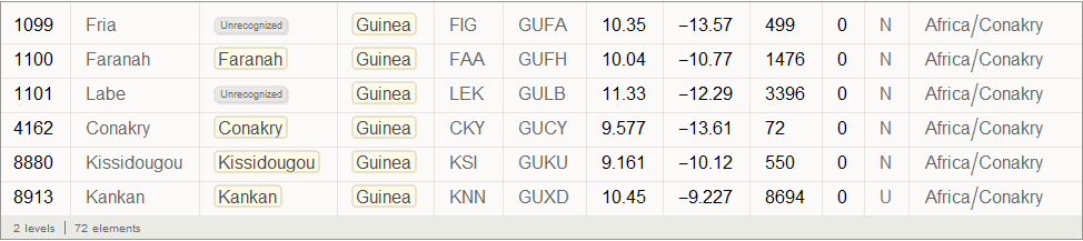
Vitali: Obtained after the function of the objects circled in orange frame with a light orange background are the so-called Entity , appeared in Mathematica 10. They are, in fact, the keys of centralized access to Wolfram | Alpha databases.

In [17]: =



Out [17] =



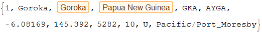
So, we see that the SemanticImport function automatically classified the third and fourth data columns as cities and countries, presenting them as Entity objects.

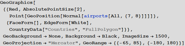
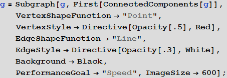
Marco: Now we can display all the airports of the World.

Vitali: Indeed, with the new features provided by the geographic computing sublanguage functions, in particular, using the GeoGraphics function and its many options, such as GeoBackground , GeoProjection and GeoRange , we can create an image that allows you to easily display a large data array.

In [18]: =



Out [18] =



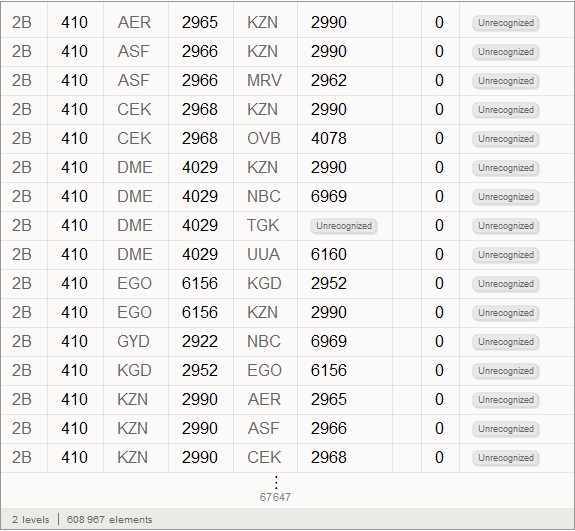
The fifth column in the airports database is the three-letter IATA (International Air Transport Association) identifier. We will need these identifiers to define the routes between the airports, which are stored in the second database. Not all the records in the airports database have them, say, below you can see the values ​​of the last 100 records of the base from the corresponding column.

In [19]: =



Out [19] =



Some of them are incorrect due to the fact that they contain numbers. We will clear our data by deleting records with incorrect or missing IATA identifier. Below you can see the number of records in the source database.

In [20]: =



Out [20] =



Now clear the database and overwrite it. The number below shows, again, the number of records, but already in the updated database.

In [21]: =



Out [22] =



Marco: Now we will create a list of rules linking airport identifiers and their geo-coordinates.

In [23]: =



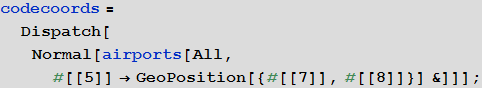
Vitali: We used the Dispatch function, which creates an optimized representation of the list of replacement rules, which does not affect the results in any way, but allows us to work with long lists much faster.

Marco: Now we can analyze the connections between airports. The number below shows the total number.

In [24]: =



Out [25] =



Not every IATA identifier has geo-coordinates, so we’ll clear the list of links between airports by deleting links without information about airport geo-coordinates.

In [26]: =



Out [27] =



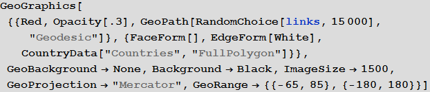
In general, 67,210 links turned out. In the figure below, we will display only 15,000 randomly selected of them, so that the main directions of flights can be disassembled.

In [28]: =



Out [28] =



Vitali: Now that we have data, how to integrate them into mathematical models?

Marco: We need to describe the paths of population movement. We will use the global air transport network to build the first pandemic model. We will consider flights as links between different areas. These areas can be considered as the “population basins” of the respective airports.

Vitali: You can use the Graph function to create graphs quickly and efficiently. There are many different connections between the same airports, so the resulting graph will be a multigraph, the latest version of the Wolfram Language has just added functionality to work with them. , , , , . , , .

In[29]:=



IATA.

, , . , .

In[30]:=



Out[30]=



In[31]:=



In[32]:=



Out[32]=



.

In[33]:=



Out[34]=



: (i, j) , i j , . SparseArray . « » , . , , , .

In[35]:=



. , . , «» . , :

• . , , , . , , : , , , . , :

In[37]:=



• . . , . , , , , . , :

In[38]:=



. - .

• . , ( ) . , , . , , , . - . (compartmental population model), , , , . ( , , ) , , , . ( ), . ( ), :

In[39]:=



, — — : , . , , , . , , , , , . .

, :

In[40]:=



5% , .

: 2013 , -. The New York Times , , , -. . :

In[41]:=



Out[41]=



, ( CKY), :

In[42]:=



Out[42]=



In[43]:=



: , SIR- , , , — () :

In[46]:=



— , :

In[47]:=



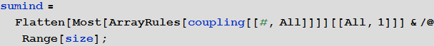
, , sumind . SIR-:

In[48]:=



, . , . .

:

In[50]:=



Out[50]=



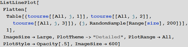
, S , I R 200 :

In[51]:=



Out[51]=



:

In[52]:=



Out[52]=



, :

In[53]:=



, :

In[54]:=



Out[54]//TableForm=












, ( ).

In[55]:=



Out[55]=



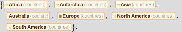
, : , , . . Graph.

: Graph , . (. ) Entities. , CTRL + SHIFT + =, «continents» .

In[56]:=



, , , :

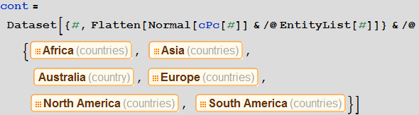
In[57]:=



In[58]:=



Out[58]=



, , , :

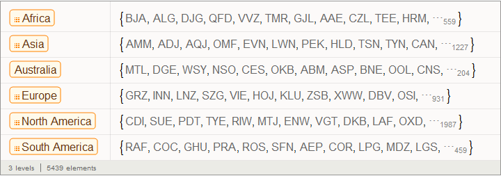
In[59]:=



:

In[61]:=



Out[61]=



() (graph communities), :

In[62]:=



Out[63]=



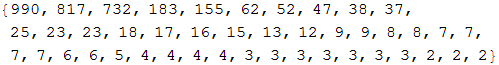
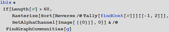
— , , , , . , , , 60. :

In[64]:=



Out[64]=



, . , :

In[65]:=



Out[65]=



: . , . . , , :

In[66]:=



In[67]:=



In[68]:=



Out[68]//TableForm=












: «RadialEmbedding» GraphLayout ( ) «RootVertex» ( ), «FNA», . . , . , . , , ?

: , . , , . , , , . . , , , .

: ?

: , SIR- SIR-, . , , . :

1. , , .

2. , , .

3. (/ ) . , : , , - .

4. / , ; , .

, . , . , . , , , , .

( ) . . , .

, , :

In[69]:=



In[70]:=



SemanticImport , . « » > «»:

In[71]:=



Graph. , :

In[72]:=



: , , ?

: , , . , , , . , , , , — , . .

, , , . , :

In[73]:=



, , ( ) :

In[74]:=



, :

In[75]:=



, , . , , . , , .

, :

In[76]:=



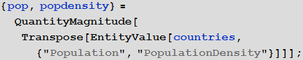
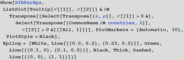
«» , () . ρ = 0.2. «» , , . , . , «» — — , . , , λ ρ ( , ) , , .

:

In[77]:=



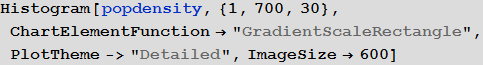
Out[77]=



:

In[78]:=



Out[78]=



, . « » , 0.2. , , :

In[79]:=



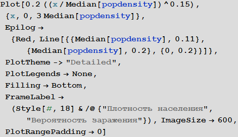
Out[79]=



:

In[80]:=



, «» . , ?

: , , . , . , , , , . « » - . . ?

: , . , , , ( «»). , , 0.5. , , 0.5. . " The scaling of contact rates with population density for the infectious disease models " by Hu et al., 2013, , , .

, . , , . , , Mathematica .

In[82]:=



:

In[83]:=



Out[83]=



, , 70 . , , ( ) .

:

In[84]:=



Out[84]=



, , , , , , . , , , :

In[85]:=



Out[85]=



, :

In[86]:=



, . , . , , , SIR- (. ).

In[88]:=



Out[88]=



: , . , , , , . , — . , , , , , . , , , — .

, , ?

: : . , , . . . ( / ) — . , -, . : , . : , . . , , , , . , « » . , , . , , , .

: , , . . .

: , , , , . , . / , ! , , , . , ; . , .

In[89]:=



, , « ».

In[92]:=



, , :

In[93]:=



- (), , :

In[95]:=



Out[95]=



:

In[96]:=



, , , :

In[99]:=



In[101]:=



:

In[103]:=



Out[103]=



, , — , :

In[104]:=



Out[104]=



, , . , . :

In[105]:=



Out[107]=


, . .

In[108]:=



Out[108]=



In[109]:=



Out[109]//TableForm=







, . — . , , , , . ; . , , «». , . , , - .

, , . , , , . , . , (, , , , , , - ). ( ) , .

: . , , , , :

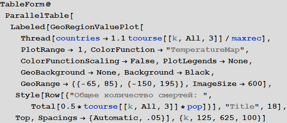
In[110]:=



:




, , . The New York Times « ? » (CDC) , () .

, , ?

: , , , , , Hu . . Mathematica (, ) . . , , . , , ?, ?, ?, / .

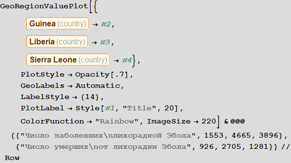
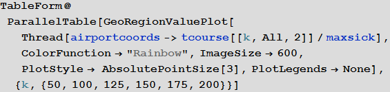
: , ListLinePlot GeoRegionValuePlot, , . , , , , . . , , (Dick Brockmann)?

: : , , . (Dirk Brockmann), , () . . , , , , .

: , . , - ?

: : — /, , . . . - , . SIR- , . . . «»; . . . «» , ( , ), , , , , , . , ; . . : , . , .

, . 18 , . . « » , . , , . - .

. , , , : / , , . . , , , , . , , , , , , . , , . , — , . , // . ., , , - . , , , , . . , ( , ρ~λ~1).

, ρ=1 , λ . . «» , , - , . , , (WHO). , : «» , «».

, , . , , , , . «» , . , . .

: ? , . . μ? ? / . . ; , , .

: .

Resources for learning Wolfram Language (Mathematica) in Russian: http://habrahabr.ru/post/244451