White Cube on guard of air purity, part 1
Device for monitoring the parameters of the home environment with the transfer of data over Wi-Fi.
The article describes a device for measuring, displaying on an integrated display and transferring environmental parameters to a network via Wi-Fi:
')
• CO2 level (carbon dioxide)
• CO level (carbon monoxide)
• Vapor content of ethyl alcohol (C2H5OH)
• combustible gas level (LPG)
• ammonia level (NH3)
• hydrogen content (H2)
• atmospheric pressure values
• humidity and air temperature
• light level
• magnetic field level along three axes
• gravity level along three axes
• level of acceleration along three axes
• temperature of any number of digital temperature sensors type DS18B20.
The highlight of the BC is a way to change screens by double tapping on the body. Video as it happens:
A detailed description of this control method is below.
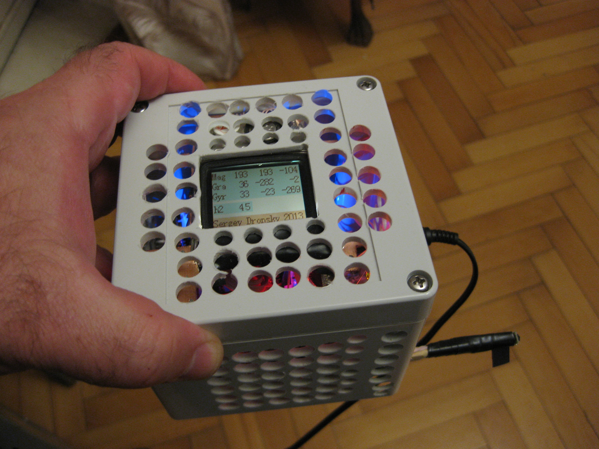
White Cube outwardly is a white body with a 10 cm edge, bought in Chip and Dipe.
When thinking about the implementation of the device, I decided that the device should give all the collected data to the network. The data is interesting not at once, but with its long-term trends. It is very interesting to have large data archives for further processing. Thus, it is reasonable to transfer data from sensors to a “big machine”, process there, store, retrieve, read statistics, draw graphs, build various correlations, etc. It only makes sense to do all this on a large machine with a powerful processor, large memory, large display and low complexity of data processing, using all the wealth of software to display and various data processing.
As a central processor, I used Arduino Nano. For me, the ease of development and programming outweighed the flaws. Considering also the noticeable power consumption of the gas sensors, the CO2 sensor and the Wi-Fi module, it does not make sense to fight for low CPU consumption. Plus, we must take into account the fact that the BC is a single device, not intended for mass production.
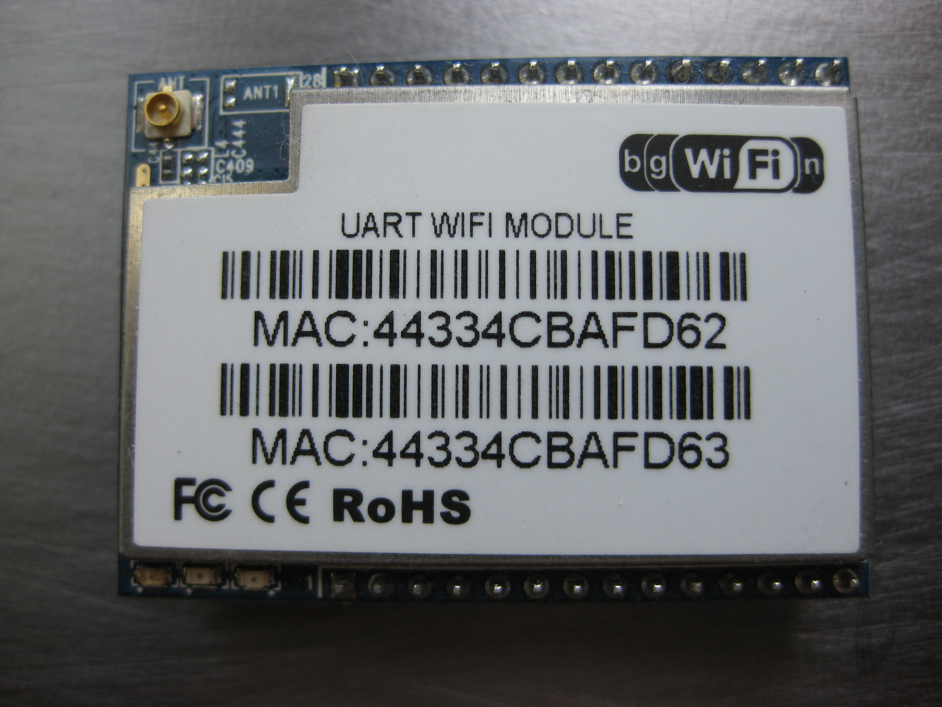
To transfer data via Wi-Fi, I used the wonderful HI-LINK HLK-RM04 Serial Port-Ethernet-Wi-Fi Adapter Module (http://dx.com/p/hi-link-hlk-rm04-serial- port-ethernet-wi-fi-adapter-module-blue-black-214540), which is essentially a mini-router with great potential.
And from the back:
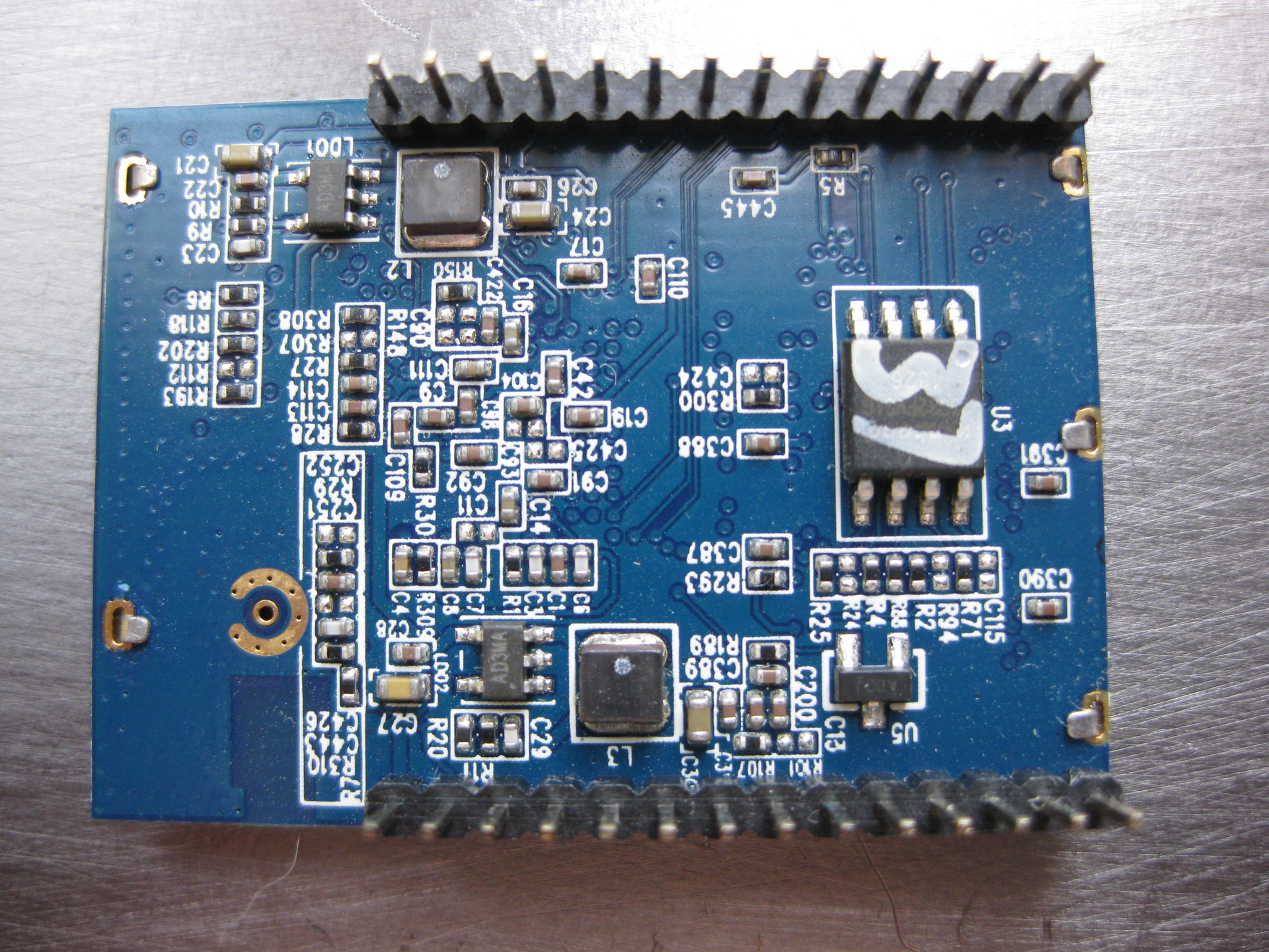
I used the transparent data transfer mode Serial - Wi-Fi. I will not dwell on this device in detail - there are enough descriptions, application experience and forums on this mini-router in the network.
From the curious one should mention the library github.com/chunlinhan/WiFiRM04
The debugging process revealed some features of data transmission over Wi-Fi compared to cable. So, if by cable a data line from for example 130 bytes from Arduino and comes in 130 bytes line, when transmitting the same line via Wi-Fi data is broken into 4-5 parts and at the receiving end these parts need to be collected and only then send a string for processing. In-depth with this, I did not understand, I took into account when writing a program for receiving data from the White Cuba. Perhaps these features of transmission over the radio channel are associated with the already heavy workload of the 2.4 GHz band and the competitive access of devices operating on the same frequency channel.
It should be noted that with DX modules come without an internal antenna:
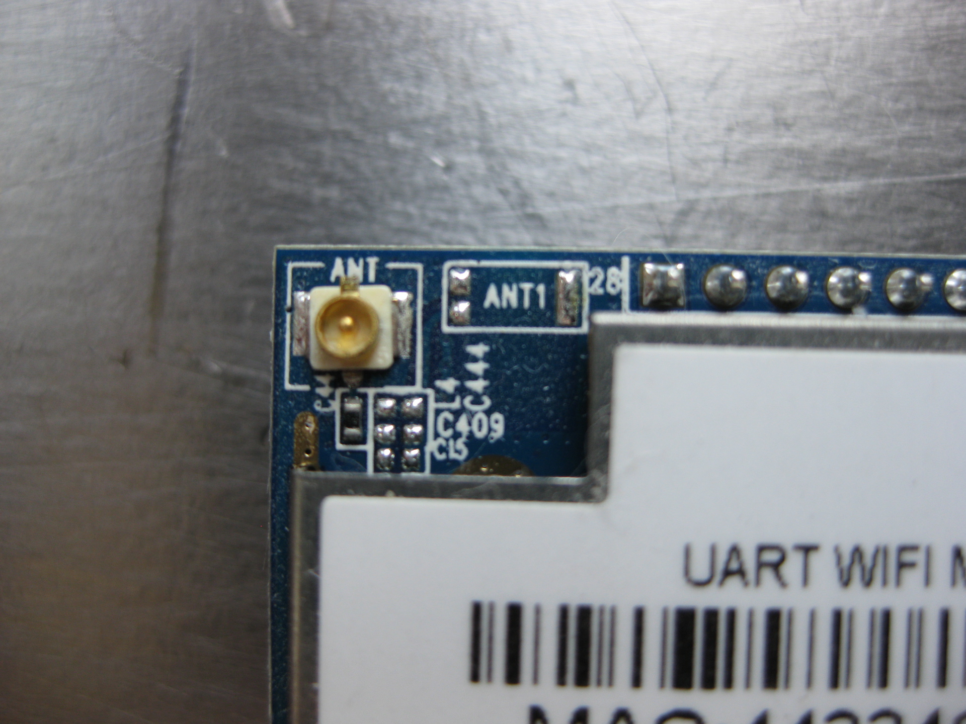
I bought external antennas in DESSY.RU and demanded reimbursement from the seller.
The following sensors are used to assess the presence of harmful substances in the air:
CO2 sensor type K-30 :
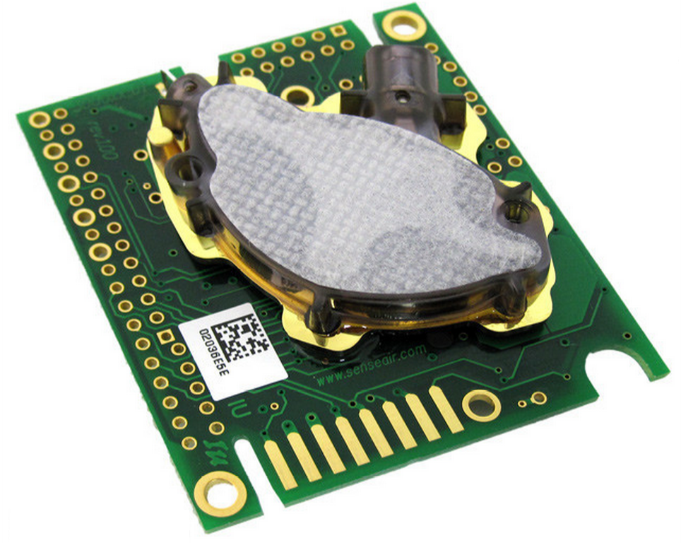
Purchased separately from the manufacturer on the site. This is the most expensive of the sensors used, but it is worth the money because it is very durable and stable. The principle of operation is to measure the absorption of infrared radiation in a calibrated path. Data from this sensor can be removed both in analog form and in two digital interfaces - serial and I2C. Also, this sensor contains an auto-calibration mechanism, which takes into account the data for the past two weeks (the time interval is programmed) and counts the minimum level during this time for 400 ppm. Thus, the long-term sensor calibration offset is taken into account. The manufacturer’s website contains both detailed documentation and examples of a data reading program, which I used. I bought two sensors, one through the serial converter - USB on the FT232 is connected to the home control machine, the second is used in the BC. The sensor is powered by 5 volts, but the levels on the serial port should be 3.3 volts. This is for the case of connection to the serial port. If I2C port is used, then a level converter is not required.
The rest of the sensors are analog:
Ethyl alcohol vapor (C2H5OH) - MQ5
CO-MQ7 carbon monoxide
Hydrogen H2 - MQ8
Liquefied Gas (LPG) - MQ6
Ammonia (NH3) - MQ135
Smoke - MQ2
The sensors look like this:
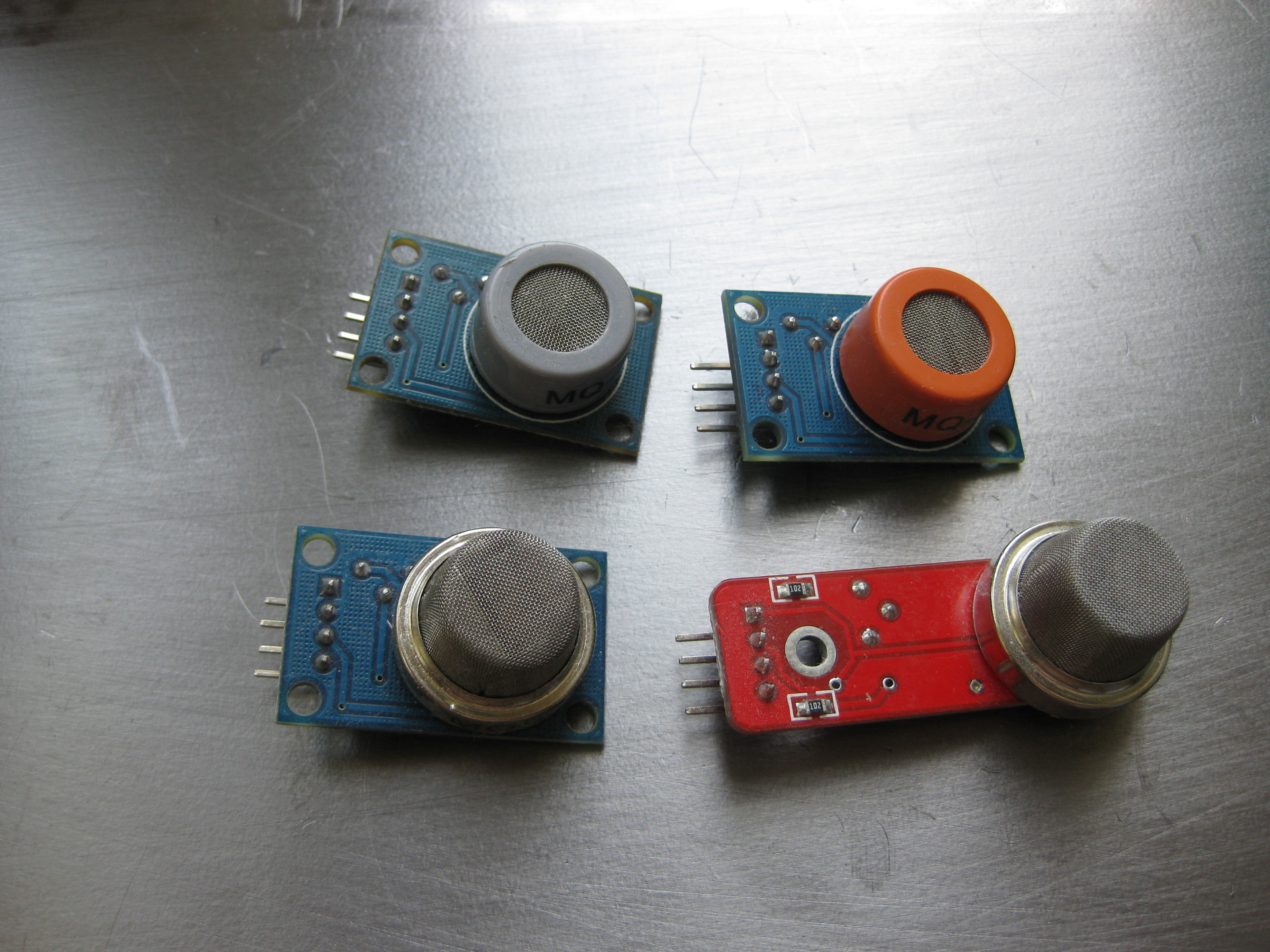
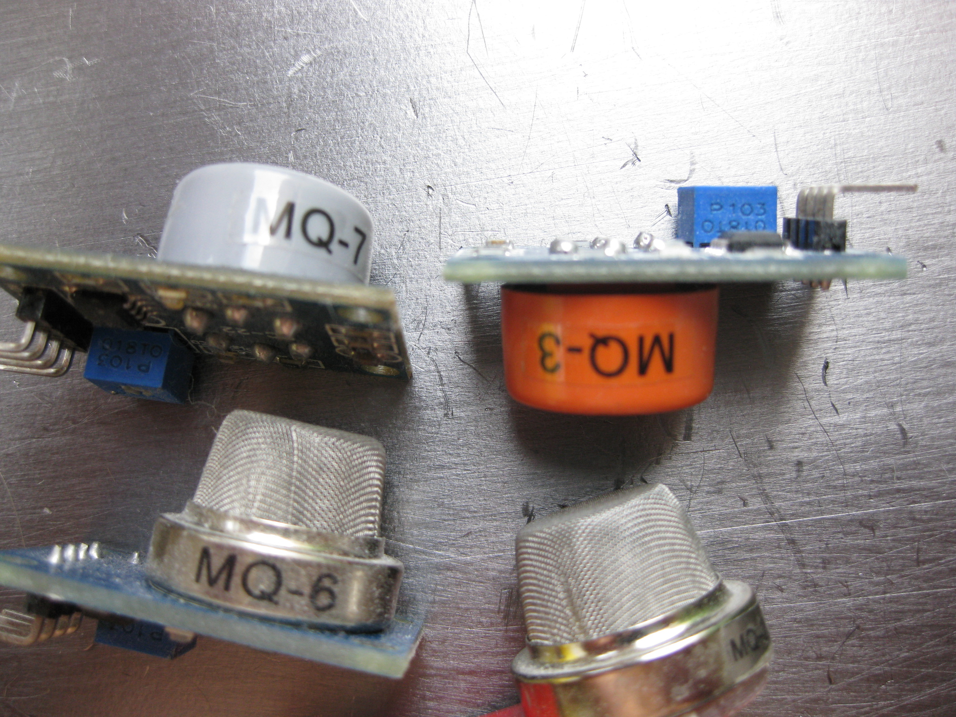
Despite some external difference, the sensors are arranged in the same way, they contain a sensitive element that changes the conductivity under the action of one or another gas and a comparator on the LM393 half. The sensors have 4 external outputs - two for powering the module (+5 and ground) and two outputs - one analog and one digital from the comparator output.
Sensitive elements require heating and therefore the current consumption is quite large - about 200 mA.
Recommended manual circuit - in series with the sensor resistor is turned on and it is removed from the useful signal. According to the manual load resistor can be set from 5 to 47 KΩ, a typical value - 10 KΩ.
It is curious to note that the sensors themselves have low selectivity and react equally well to the entire spectrum of substances and gases. This, however, became clear already in the process of testing and debugging the BC.
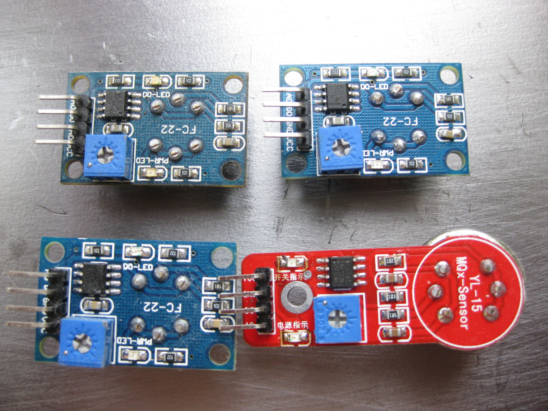
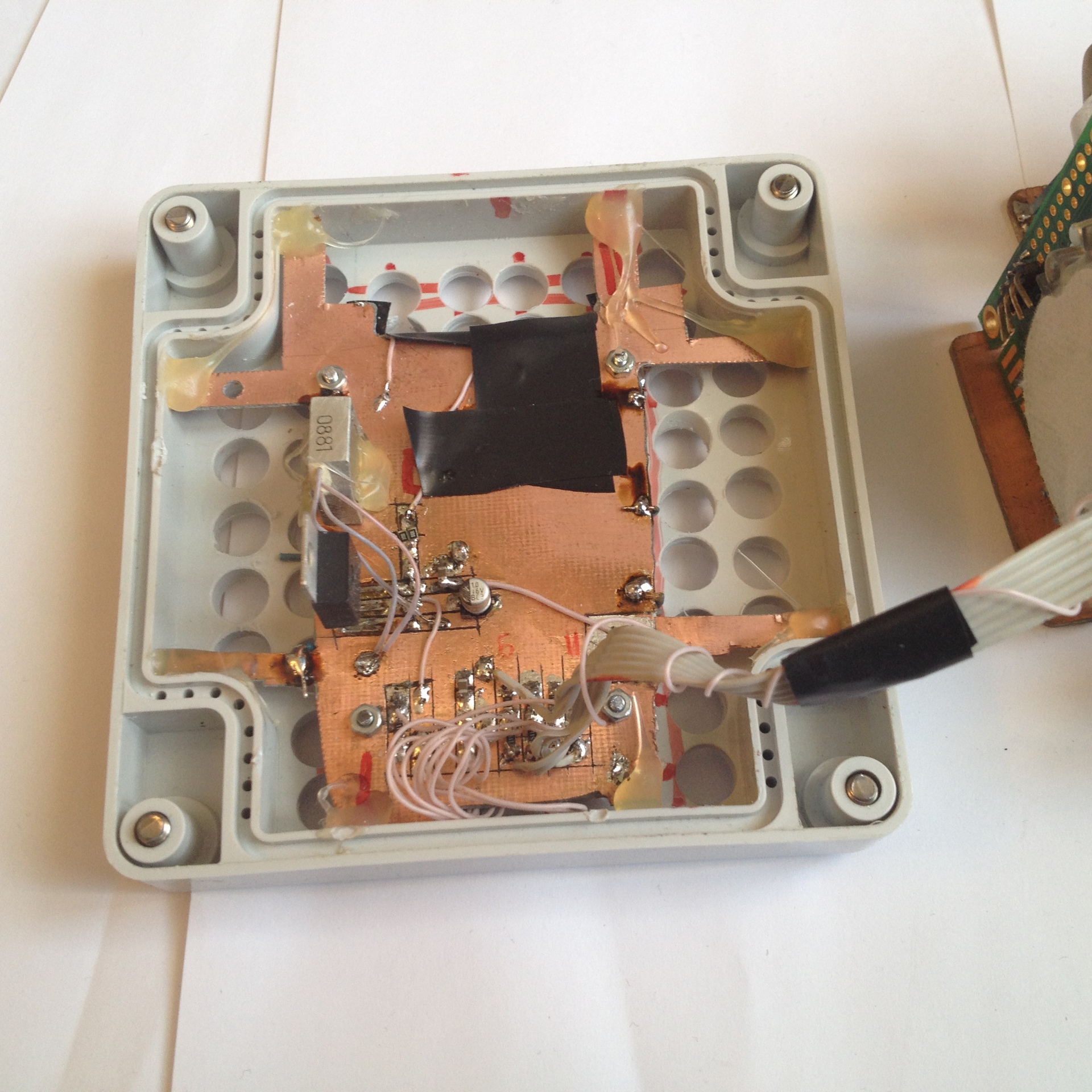
On the printed circuit board is placed the actual sensor, dual comparator type LM393, a pair of LEDs and auxiliary strapping. One LED is a power indicator, the second is a comparator trigger indicator. Fortunately, the output connector has an analog signal output directly from the sensor, so I was able to use these nodes without changes, except for the CO sensor.
CO sensor (MQ7) had to be upgraded. This sensor requires a special power mode in accordance with the manual. 90 seconds a full voltage of 5 volts should be applied to the heating element, and then 60 seconds - 1.4 volts. On the board, the heater power supply is organized differently - +5 volts are fed to one heater output, and the second output is connected to ground through a 5 ohm resistor.
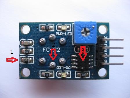
The photo shows the red arrows:
1 - 5 ohm resistor in the heater circuit
2 - heater output
3 - LM393 comparator
I dismantled the resistor (1) and connected the output of the heater (2) to the foot of the connector, to which the comparator output was connected, with the MGTF wire. I also removed the comparator (3) from the board. The second wire restores the erroneously destroyed indicator LED circuit. The indicator LED is connected in parallel with the heating element. This made it possible to visually monitor the current mode when debugging a program — heating or measurement by changing the brightness of the LED.
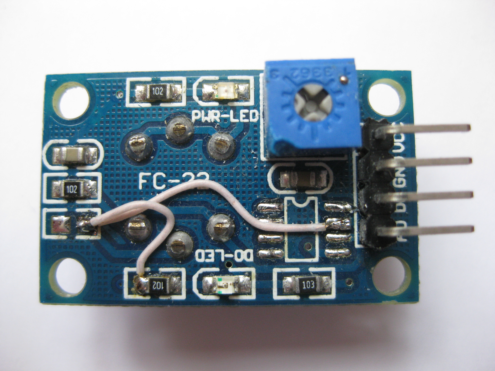
Photo of a converted CO MQ7 sensor
Since the sensor heater requires a significant current (about 200 mA), it is impossible to supply it directly from the Arduino output (maximum 40 mA). I used the intermediate field effect transistor in key mode. The transistor is like this: IRLU120NPBF, Nkan 100V 10A logic TO251, purchased in Chip and Dipe. This is a T1 transistor on the circuit diagram of the BC.
Electrical concept of White Cuba:
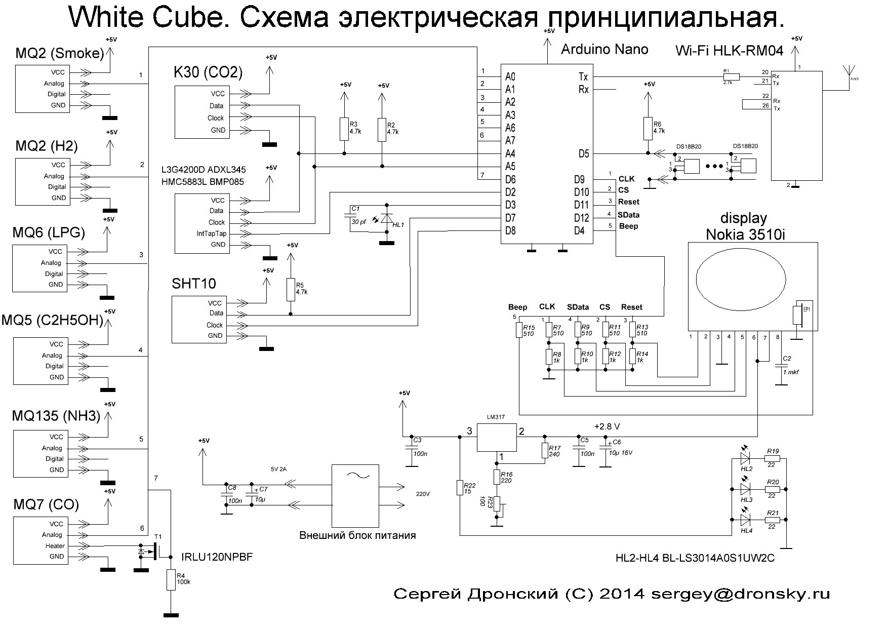
Having studied the materials on the Internet, I decided that the pulse supplying the sensor in the PWM mode of the required duty cycle would be optimal. Other methods - for example, the sequential inclusion of diodes or resistors - require manual selection of elements. The disadvantage of this method is that the pulse power of the heater can lead to interference with the measurement of the analog signal from the sensor.
Having carefully read the datasheet, I realized that the CO level should be measured at the very end of the measurement cycle immediately before turning on the heating cycle. Therefore, I decided that I would not take any special measures to suppress the impulse noise from PWM, but simply turn off the PWM signal before measuring, let the system calm down for a few milliseconds, measure the CO level and then turn on the power again. The thermal inertia of the sensor is tens of seconds, so that during switching the temperature of the sensitive element does not change and the output signal is also stable.
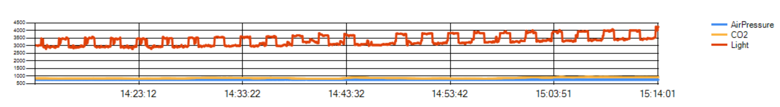
The type of output signal in the CO measurement channel is shown in the graph:
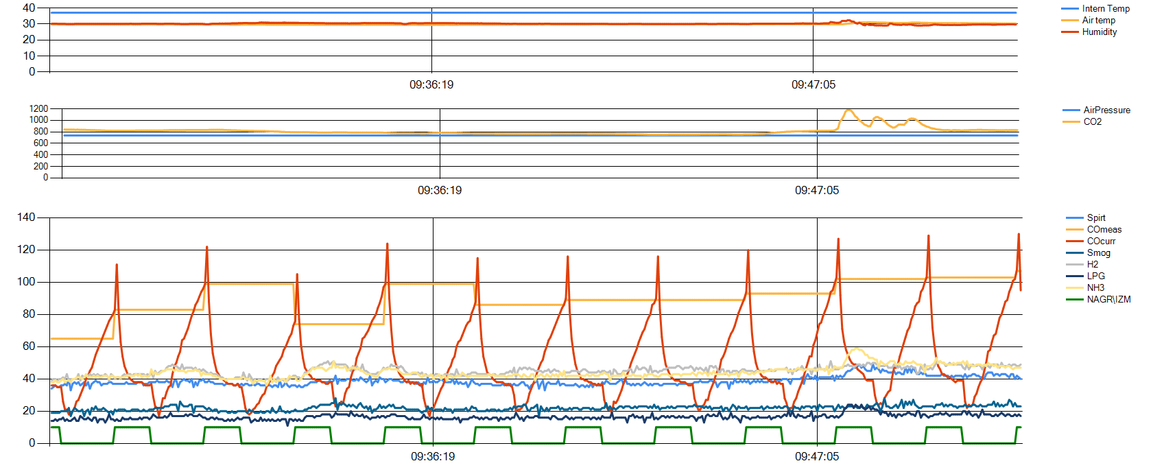
In this graph, the green meander is the switching of the voltage on the heating element, the red line is the signal from the CO sensor, the yellow one is the signal recorded just before the heating mode is changed.
The signal from the CO sensor is measured continuously, the processing system receives both the current signal, measured with a period of about 3 seconds (the period of the main sketch cycle), and measurement “by manual” with a period of 2.5 minutes (90 + 60 seconds). From the graphs it can be seen that the signal within the measurement period also carries information about the current level of CO and its rate of change. You can select and use it by comparing (subtracting) the stored array of values from the previous measurement cycle with the current values. The difference with the previous cycle with perhaps some additional processing (averaging over 10-20 seconds) will give more or less adequate information about the rate of increase of the harmful agent in the air. This will increase the speed of reaction to the change of CO from two and a half minutes to several seconds. I found the idea of such processing here .
The remaining analog sensors do not require special power. All analog gas sensors require heating for 48 hours after power is applied.
Air pressure measurement.
To measure this parameter, I used the L3G4200D ADXL345 HMC5883L BMP085 MWC Sensor Module for Arduino module.
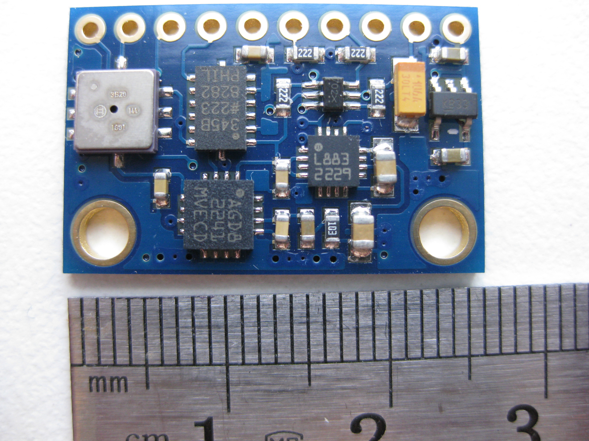
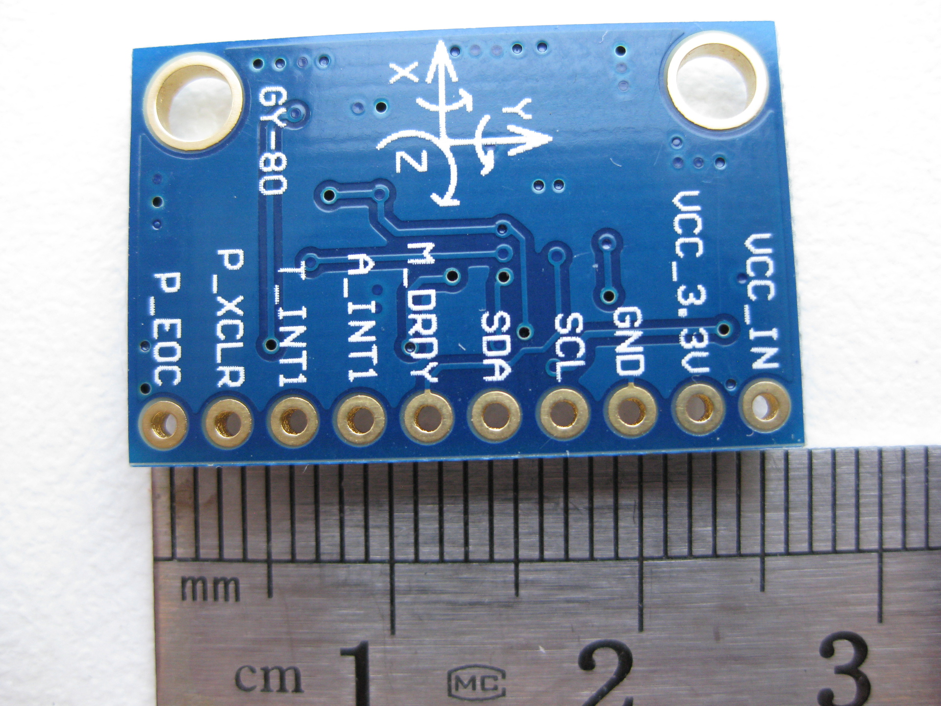
The module contains 4 sensors, originally designed for aircraft type multicopter. Module purchased on DX.com for reasons of "wholesale cheaper." It turned out, however, that the ADXL345 sensor was also used. This is somewhat lower.
BMP085 is a digital absolute air pressure sensor with a temperature sensor.
ADXL345 - three-axis acceleration sensor
HMC5883L - three-axis magnetic field sensor
L3G4200D - three-axis digital gyroscope.
All sensors are connected to the I2C bus, for reading I used ready-made libraries.
The ADXL345 sensor is designed to measure acceleration along three axes with results output via the I2C bus. This sensor can measure in particular the acceleration of gravity.
And this sensor is able to respond to the effects of “tap” and “double tap” - i.e. on single and double tapping. And this makes it possible to exert control actions on the program (sketch) of the BC. I used this mechanism to switch screens on the display. There is a lot of data and they do not fit on one screen. Therefore, I grouped them on three screens and switch them on double tap on the BC case. I really did not want to make any buttons, I wanted to leave the BC surface as clean as possible.
ADXL345 is able to set a hardware interrupt upon detection of double tap, I connected it to the Arduino D3 pin.
Unfortunately, due to the limitations of MK, I could not manage to organize a full processing of hardware interrupts. Inside the interrupt, I cannot poll the ADXL345 registers, since if the interruption happened inside the program of communication with another device on the same I2C bus, I will break this exchange. Therefore, I made a compromise - when processing an interrupt from an ADXL345, I just set the flag that double tap is registered, and I actually do the ADXL345 poll to reset the interrupt flag in the screen output routine. The solution is not perfect and sometimes gives artifacts on the screen, but as fast as possible. If you simply poll the main loop of the ADXL345 for the presence of an event - then the reaction time can be about 3 seconds in case of an unsuccessful scenario. It's annoyingly long ... My option gives a maximum delay of less than a second and I found it acceptable.
Video switching screen for double tapu:
The data from the magnetic field sensors and accelerations are read, displayed on the display (screen 2) and transmitted through the communication channel without changes. Their processing is still a matter of the future.
If you turn the cube in your hands, the readings of the acceleration sensor, gravity and magnetic field will change. There is also an active reaction in the presentation of the magnet.
What practical benefit to extract from these indications - I have not decided yet. Maybe an analysis of changes in the magnetic field will give some useful information for meteosensitive people? However, as an electronic compass device can be used now.
Light sensor.
I have a couple of free outputs on the Arduin, one of them with a hardware interrupt. I decided to use this output to measure light. In the network, I found references to the method of measuring the illumination by measuring the discharge time of the reverse-on pn junction of the LED. The essence of the method is as follows - the led turns on again at the processor output. The output switches to OUTPUT mode and a high level (+5 volts) is applied to it. The parasitic capacitance of the LED plus the mounting capacitance charges to a high level. Next, the output switches to INPUT mode and an interrupt is attached to it by a level change or by a negative edge. The input impedance of the ATMEL328P processor in this mode is quite large — tens of mega-ohms, so the discharge of the parasitic capacitance by the photocurrent takes quite a long time - from units of milliseconds to units of seconds. By triggering an interrupt, it is enough to fix the current time. The difference between the time of the beginning of the cycle and the time of the end of the cycle will give the time in milliseconds, inversely proportional to the illumination. In my case, for darkness at night, the time is about 3,500 milliseconds, and in the afternoon on the Sun - a few milliseconds. I put an additional capacitor parallel to the LED with a capacity of ten picofarads, otherwise the discharge during the day was very fast (less than 1 ms). I received 3-10 ms on a bright sunny day. Own capacitance of the LED is about 8 pF. Additional capacity has led to a noticeable increase in discharge time in the dark - more than 4 seconds. Then I ran into a certain difficulty. The main cycle of the program lasts about 3.6 seconds. At the beginning of the cycle, I start the luminance measurement, perform all other operations, and by the end of the cycle, I expect that the global variable contains the luminance value set in the interrupt. At first I had the idea to organize an autonomous cycle of measuring illumination, so that in the interruption itself the cycle would start again. But then, at high levels of illumination (i.e., a small cycle time — a few milliseconds), the processor will be busy only with measuring illumination. If you start once at the beginning of the main cycle, then at low light levels the response will not be yet and the value will be 0 ... I went out of position so - I start the measurement at the beginning of the cycle, but I check if it was triggered or not. If it was - run in a regular manner. If not, I do not do anything. The disadvantage of this solution is that at low light levels, the measurement speed drops by half. However - I am still interested in data with a characteristic change time of tens of seconds, so this minus is not important. The result was a converter of illumination to an impulse length with some features and a price of 20 rubles.
LED selection. Since by the time the illumination sensor was connected, the White Cube already had holes with a diameter of 8 mm - I decided that it would be nice to use a diode of the same diameter. I bought in Chip and Dipe a pair of pieces of LEDs of each color available there (red, green, yellow, white and blue) with a diameter of 8 mm and set up an experiment to determine the optimal LED. To study the LEDs, I built a simple stand. The stand consists of the Arduino Nano, the Wi-Fi-serial module and the LED under study on screw terminals. The system was powered from a lithium battery (power pack).
It is a little theory - the illumination in a room changes about 1000 times or more. At night, the illumination amounts to units and lumen fractions, on a sunny day, about 1000 lumens of light inside the room, and about 10,000 lumens by the window.
For each LED, I looked for the maximum illumination — it led the system in small steps to the brightest spot on the street and the darkest in the room and then carried the system into a dark room.
The results of processing measurements are shown in the table.
(numbers in the table - discharge time in milliseconds)
It turned out that the green LED has a maximum width of the range - more than 1000 times (from ms units to 4 seconds), followed by white (635 times), then red (442) and yellow (72) and the list is blue with a range of 11. White The LED was also less sensitive to light.
Detailed interpretation of the results obtained is beyond the scope of this article, but it is clear that it is optimal to use a green LED in the PC.
Converting light sensor readings to suites.
Illumination standards are easily found on the Internet (Sanitary Regulations and Standards SanPiN 2.2.1 / 2.1.1.1278-03). From the study of this document, it follows that the illumination is normalized in the range of 20 - 750 lux (from the storeroom to the workplace for precision work). In other words, calibrating the BC light sensor has a practical meaning in the range from luxury units to thousand lux.
To solve this problem, I applied a ready calibrated sensor BH1750. The sensor was connected to a separate Arduino connected to a Wi-Fi module. The sketch read the sensor readings and transmitted them to the network, from where they were taken by the program, averaged over the interval of 1 minute and recorded in the log file. After several days, I processed these primary data, comparing the data from the BC and the calibrated sensor. As a result of data processing, I received a conversion table, according to which the discharge time of the diode can be recalculated into suites. From the table, you can derive a formula, but I left it on When I'm sixty four.
The described method of measuring illumination was very sensitive to changes in the supply voltage and other destabilizing factors. The reason for this is that the output signal relies on an analog comparison operation of a very slowly varying input voltage and a reference voltage, approximately equal to half the supply voltage. It turns out that the switching time of a logic element is very strongly dependent on random fluctuations of the supply voltage, etc. Here in this illustration you can clearly see the dependence of the measured time on the supply voltage:
The supply voltage varies due to the heating and measuring cycles of the CO MQ7 sensor. In the measurement cycle, 1.4V is supplied to it, and in the heating cycle - 5V, the current consumption changes, the supply voltage changes, and the response threshold of the D3 floats. According to the measurements, it turned out that due to the factor of instability in the power supply, the time change is from 10% at high light levels to more than 30% at low levels.
This change can be corrected programmatically.
Considering that the measurement accuracy turned out to be quite low (errors of the order of 30%), I decided to limit myself to the simplest way of converting the measured discharge time into lux in a table. The microprocessor Arduino Nano has very modest resources for serious processing of such data, and I decided to transfer more serious processing to a Visual Basic program. In such a program, you can filter the data, averaging over a large time interval. At the moment, the schedule of illumination per day looks like this:

Black arrow - the moment when the TV is turned off Red is the sunrise (today, November 20, 2014, it is 8:13 according to Gismeteo).
The sensor in the form of a diode saves responsiveness to low levels of illumination in the area of units and tenths of a lux. The BH1750 sensor has a minimum sensitivity of 1 lux. For example, the BH1750 does not respond to a TV or a desk lamp with a unit power of watts (LED), and the sensor in the BC reacts with confidence. There are, however, other light sensors with a significantly large range, for example, the MAX44009 with the stated range of 0.045 - 188000 lux, I2C interface, but also at the price of about 200 r (in Chip and Dipe - 250r). However, maybe in the next version of BC I will replace the light sensor. The use of ready-made modules is certainly more correct in terms of the quality of the end product, but it’s more interesting to do something with your own hands.
Using the LED and the method of measuring the discharge duration in such a simple form does not provide sufficient accuracy, but can be used, for example, to perform a display brightness adjustment or some other tasks that need to know the illumination roughly, with an accuracy of 30-40%. Let us say perhaps the confident distinction of day and night.
Display
In BC, I used the display from Nokia 3510i. Its only advantage is a very low price in the stores of spare parts for cellular. I bought this display for 46 p. Minus - there are no backlight LEDs, you need to make your own, small size, small chromaticity - 4096 colors and confused exchange programming in 4096 colors. At the moment, the best seems to be the use of ready-made modules like this . This module is somewhat more expensive (about 300 p), but the full color, built-in lights, simple programming outweigh the slight increase in price. I used this module in the radiometer and am quite pleased with its quality. About the radiometer with Wi-Fi and Glonass \ GPS, see the article here .
I made the backlight in the display of the Nokia 3510i in the form of a strip of double-sided foil fiberglass with evenly placed three LEDs. The height of the bar is about 3 mm, width - corresponds to the width of the end of the display. The slit is made in the foil and the LEDs are soldered in place. A resistor of 20 ohms is connected in series with each diode, all sections are connected in parallel, and another resistor is connected in series to control the backlight brightness. The bar is soldered with two copper wires in the end of the display. The suspension of the backlight on flexible copper wires allows you to adjust the position of the strip for optimal display brightness.
LEDs “BL-LS3014A0S1UW2C, LED SMD 3014, Warm White, 120˚ 2300mKd”, bought in Chip and Dipa at 26 p. Taking into account the LEDs (3 used + 1 burned), the price of the display is about 150 rubles, which is only half as much as the finished one.
The display module is mounted in the cube cover and attached to the main module with a flat cable. Additional wire - to connect the speaker, which is on the display. I used it at the last moment, when there was both a free leg on Arduin and a place in memory for the code that generates sound signals.
The strange form of the display module was due to design errors. I decided that the holes on the sides of the cube would be enough to dissipate heat, but it turned out that there was not enough and it was necessary to make holes on top too. Since the display module covered the entire top cover, it was necessary to remove everything possible to give the maximum passage for warm air. Scissors for metal and Dremel perfectly coped with the task of removing unnecessary :) Additional wire MGTF, wrapped around a flat cable, added at the last moment to give a signal to the squeaker.
Built-in BC display, screen 1:
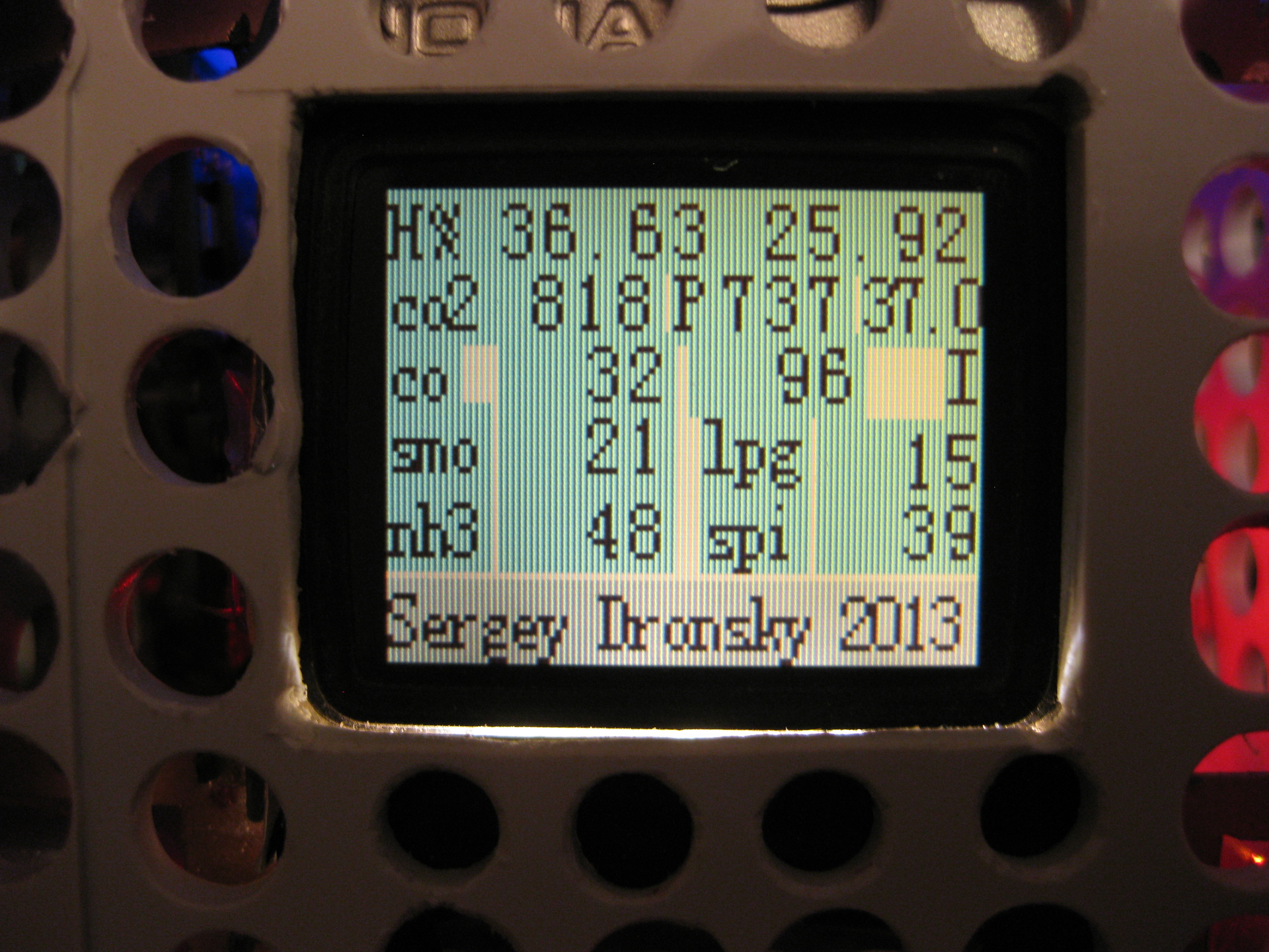
From left to right, in the following lines:
Humidity, air temperature
CO2 level, ppm, air pressure in millimeters of mercury, air temperature inside BC
CO level current, measured, status (N - heating, I - measurement)
Smoke level, level of combustible gases
Ammonia level, ethyl alcohol vapor
Screen 2:
From left to right, in rows:
Magnetic field sensor readings on three axes - X, Y, Z
The indications of the gravity sensor on the three axes - X, Y, Z The
indications of the acceleration field sensor on the three axes - X, Y, Z
The level of hydrogen, the illumination.
The last value in the first line is actually a deviation from the direction to the north magnetic pole.
Here is a curious picture:
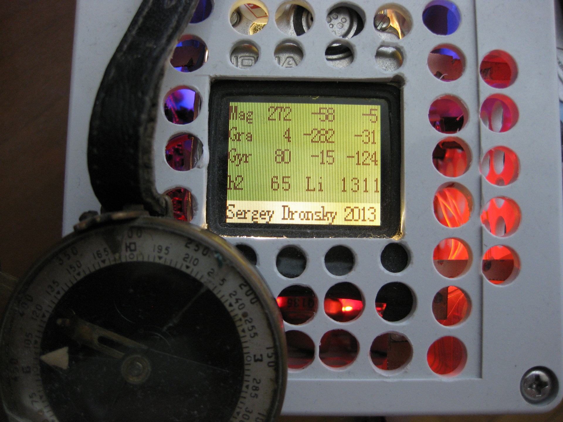
As you can see, the compass needle and the face of the cube are almost parallel to each other and the direction to magnetic north.
Zero axis Z - because the sensor is installed vertically and the Z axis is horizontal, the Y axis is vertical.
Screen 3, temperature sensors:
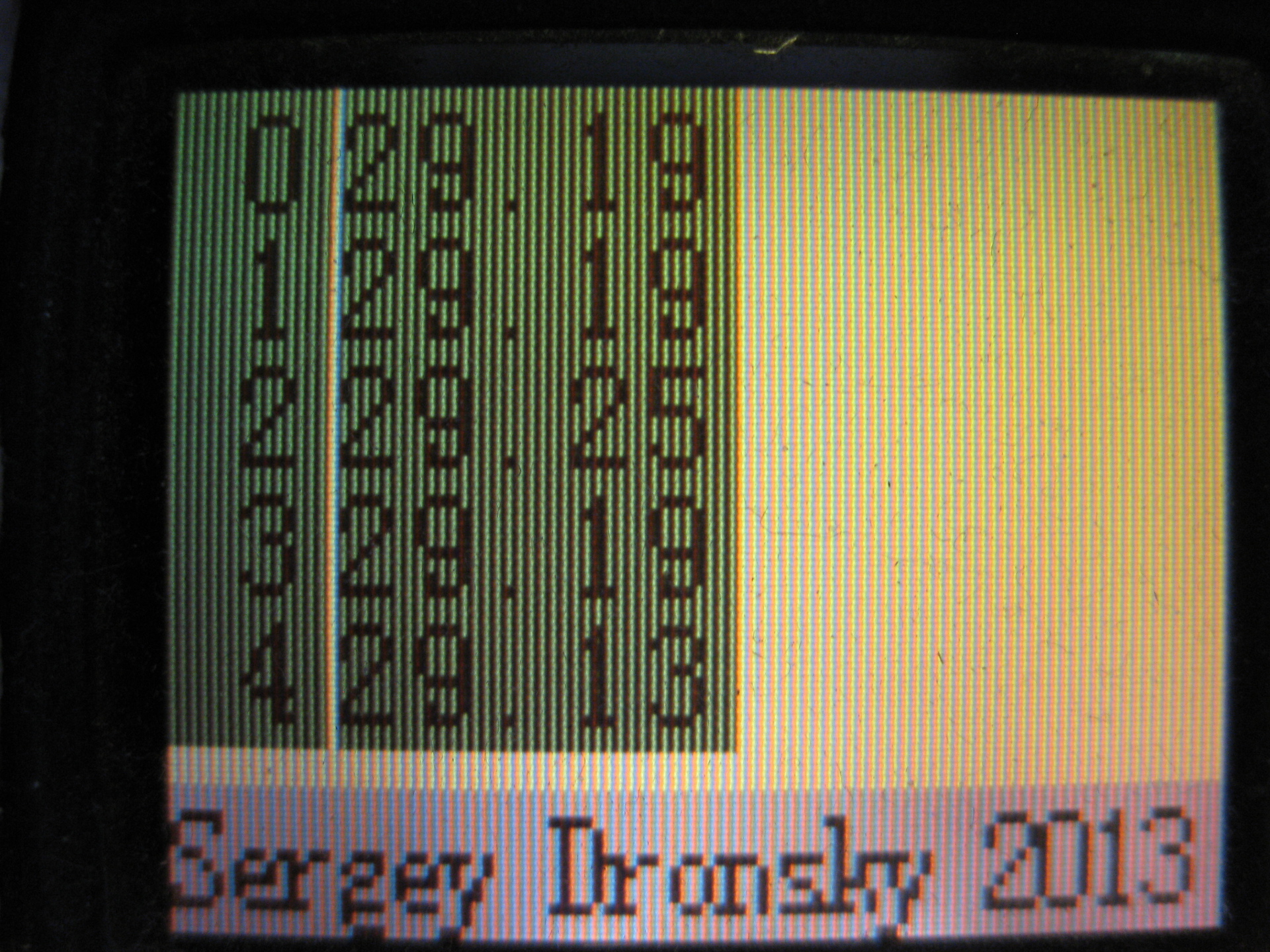
A loop of five Dallas 18B20 sensors is connected to Cuba, the sketch at start determines the number of connected sensors and only polls them during further operation.
Here is a video of the launch of the sketch, which smoothly changes the brightness of each of their primary display colors at the start:
To be continued .
The article describes a device for measuring, displaying on an integrated display and transferring environmental parameters to a network via Wi-Fi:
')
• CO2 level (carbon dioxide)
• CO level (carbon monoxide)
• Vapor content of ethyl alcohol (C2H5OH)
• combustible gas level (LPG)
• ammonia level (NH3)
• hydrogen content (H2)
• atmospheric pressure values
• humidity and air temperature
• light level
• magnetic field level along three axes
• gravity level along three axes
• level of acceleration along three axes
• temperature of any number of digital temperature sensors type DS18B20.
The highlight of the BC is a way to change screens by double tapping on the body. Video as it happens:
A detailed description of this control method is below.
White Cube outwardly is a white body with a 10 cm edge, bought in Chip and Dipe.
When thinking about the implementation of the device, I decided that the device should give all the collected data to the network. The data is interesting not at once, but with its long-term trends. It is very interesting to have large data archives for further processing. Thus, it is reasonable to transfer data from sensors to a “big machine”, process there, store, retrieve, read statistics, draw graphs, build various correlations, etc. It only makes sense to do all this on a large machine with a powerful processor, large memory, large display and low complexity of data processing, using all the wealth of software to display and various data processing.
As a central processor, I used Arduino Nano. For me, the ease of development and programming outweighed the flaws. Considering also the noticeable power consumption of the gas sensors, the CO2 sensor and the Wi-Fi module, it does not make sense to fight for low CPU consumption. Plus, we must take into account the fact that the BC is a single device, not intended for mass production.
To transfer data via Wi-Fi, I used the wonderful HI-LINK HLK-RM04 Serial Port-Ethernet-Wi-Fi Adapter Module (http://dx.com/p/hi-link-hlk-rm04-serial- port-ethernet-wi-fi-adapter-module-blue-black-214540), which is essentially a mini-router with great potential.
And from the back:
I used the transparent data transfer mode Serial - Wi-Fi. I will not dwell on this device in detail - there are enough descriptions, application experience and forums on this mini-router in the network.
From the curious one should mention the library github.com/chunlinhan/WiFiRM04
The debugging process revealed some features of data transmission over Wi-Fi compared to cable. So, if by cable a data line from for example 130 bytes from Arduino and comes in 130 bytes line, when transmitting the same line via Wi-Fi data is broken into 4-5 parts and at the receiving end these parts need to be collected and only then send a string for processing. In-depth with this, I did not understand, I took into account when writing a program for receiving data from the White Cuba. Perhaps these features of transmission over the radio channel are associated with the already heavy workload of the 2.4 GHz band and the competitive access of devices operating on the same frequency channel.
It should be noted that with DX modules come without an internal antenna:
I bought external antennas in DESSY.RU and demanded reimbursement from the seller.
The following sensors are used to assess the presence of harmful substances in the air:
CO2 sensor type K-30 :
Purchased separately from the manufacturer on the site. This is the most expensive of the sensors used, but it is worth the money because it is very durable and stable. The principle of operation is to measure the absorption of infrared radiation in a calibrated path. Data from this sensor can be removed both in analog form and in two digital interfaces - serial and I2C. Also, this sensor contains an auto-calibration mechanism, which takes into account the data for the past two weeks (the time interval is programmed) and counts the minimum level during this time for 400 ppm. Thus, the long-term sensor calibration offset is taken into account. The manufacturer’s website contains both detailed documentation and examples of a data reading program, which I used. I bought two sensors, one through the serial converter - USB on the FT232 is connected to the home control machine, the second is used in the BC. The sensor is powered by 5 volts, but the levels on the serial port should be 3.3 volts. This is for the case of connection to the serial port. If I2C port is used, then a level converter is not required.
The rest of the sensors are analog:
Ethyl alcohol vapor (C2H5OH) - MQ5
CO-MQ7 carbon monoxide
Hydrogen H2 - MQ8
Liquefied Gas (LPG) - MQ6
Ammonia (NH3) - MQ135
Smoke - MQ2
The sensors look like this:
Despite some external difference, the sensors are arranged in the same way, they contain a sensitive element that changes the conductivity under the action of one or another gas and a comparator on the LM393 half. The sensors have 4 external outputs - two for powering the module (+5 and ground) and two outputs - one analog and one digital from the comparator output.
Sensitive elements require heating and therefore the current consumption is quite large - about 200 mA.
Recommended manual circuit - in series with the sensor resistor is turned on and it is removed from the useful signal. According to the manual load resistor can be set from 5 to 47 KΩ, a typical value - 10 KΩ.
It is curious to note that the sensors themselves have low selectivity and react equally well to the entire spectrum of substances and gases. This, however, became clear already in the process of testing and debugging the BC.
On the printed circuit board is placed the actual sensor, dual comparator type LM393, a pair of LEDs and auxiliary strapping. One LED is a power indicator, the second is a comparator trigger indicator. Fortunately, the output connector has an analog signal output directly from the sensor, so I was able to use these nodes without changes, except for the CO sensor.
CO sensor (MQ7) had to be upgraded. This sensor requires a special power mode in accordance with the manual. 90 seconds a full voltage of 5 volts should be applied to the heating element, and then 60 seconds - 1.4 volts. On the board, the heater power supply is organized differently - +5 volts are fed to one heater output, and the second output is connected to ground through a 5 ohm resistor.
The photo shows the red arrows:
1 - 5 ohm resistor in the heater circuit
2 - heater output
3 - LM393 comparator
I dismantled the resistor (1) and connected the output of the heater (2) to the foot of the connector, to which the comparator output was connected, with the MGTF wire. I also removed the comparator (3) from the board. The second wire restores the erroneously destroyed indicator LED circuit. The indicator LED is connected in parallel with the heating element. This made it possible to visually monitor the current mode when debugging a program — heating or measurement by changing the brightness of the LED.
Photo of a converted CO MQ7 sensor
Since the sensor heater requires a significant current (about 200 mA), it is impossible to supply it directly from the Arduino output (maximum 40 mA). I used the intermediate field effect transistor in key mode. The transistor is like this: IRLU120NPBF, Nkan 100V 10A logic TO251, purchased in Chip and Dipe. This is a T1 transistor on the circuit diagram of the BC.
Electrical concept of White Cuba:
Having studied the materials on the Internet, I decided that the pulse supplying the sensor in the PWM mode of the required duty cycle would be optimal. Other methods - for example, the sequential inclusion of diodes or resistors - require manual selection of elements. The disadvantage of this method is that the pulse power of the heater can lead to interference with the measurement of the analog signal from the sensor.
Having carefully read the datasheet, I realized that the CO level should be measured at the very end of the measurement cycle immediately before turning on the heating cycle. Therefore, I decided that I would not take any special measures to suppress the impulse noise from PWM, but simply turn off the PWM signal before measuring, let the system calm down for a few milliseconds, measure the CO level and then turn on the power again. The thermal inertia of the sensor is tens of seconds, so that during switching the temperature of the sensitive element does not change and the output signal is also stable.
The type of output signal in the CO measurement channel is shown in the graph:
In this graph, the green meander is the switching of the voltage on the heating element, the red line is the signal from the CO sensor, the yellow one is the signal recorded just before the heating mode is changed.
The signal from the CO sensor is measured continuously, the processing system receives both the current signal, measured with a period of about 3 seconds (the period of the main sketch cycle), and measurement “by manual” with a period of 2.5 minutes (90 + 60 seconds). From the graphs it can be seen that the signal within the measurement period also carries information about the current level of CO and its rate of change. You can select and use it by comparing (subtracting) the stored array of values from the previous measurement cycle with the current values. The difference with the previous cycle with perhaps some additional processing (averaging over 10-20 seconds) will give more or less adequate information about the rate of increase of the harmful agent in the air. This will increase the speed of reaction to the change of CO from two and a half minutes to several seconds. I found the idea of such processing here .
The remaining analog sensors do not require special power. All analog gas sensors require heating for 48 hours after power is applied.
Air pressure measurement.
To measure this parameter, I used the L3G4200D ADXL345 HMC5883L BMP085 MWC Sensor Module for Arduino module.
The module contains 4 sensors, originally designed for aircraft type multicopter. Module purchased on DX.com for reasons of "wholesale cheaper." It turned out, however, that the ADXL345 sensor was also used. This is somewhat lower.
BMP085 is a digital absolute air pressure sensor with a temperature sensor.
ADXL345 - three-axis acceleration sensor
HMC5883L - three-axis magnetic field sensor
L3G4200D - three-axis digital gyroscope.
All sensors are connected to the I2C bus, for reading I used ready-made libraries.
The ADXL345 sensor is designed to measure acceleration along three axes with results output via the I2C bus. This sensor can measure in particular the acceleration of gravity.
And this sensor is able to respond to the effects of “tap” and “double tap” - i.e. on single and double tapping. And this makes it possible to exert control actions on the program (sketch) of the BC. I used this mechanism to switch screens on the display. There is a lot of data and they do not fit on one screen. Therefore, I grouped them on three screens and switch them on double tap on the BC case. I really did not want to make any buttons, I wanted to leave the BC surface as clean as possible.
ADXL345 is able to set a hardware interrupt upon detection of double tap, I connected it to the Arduino D3 pin.
Unfortunately, due to the limitations of MK, I could not manage to organize a full processing of hardware interrupts. Inside the interrupt, I cannot poll the ADXL345 registers, since if the interruption happened inside the program of communication with another device on the same I2C bus, I will break this exchange. Therefore, I made a compromise - when processing an interrupt from an ADXL345, I just set the flag that double tap is registered, and I actually do the ADXL345 poll to reset the interrupt flag in the screen output routine. The solution is not perfect and sometimes gives artifacts on the screen, but as fast as possible. If you simply poll the main loop of the ADXL345 for the presence of an event - then the reaction time can be about 3 seconds in case of an unsuccessful scenario. It's annoyingly long ... My option gives a maximum delay of less than a second and I found it acceptable.
Video switching screen for double tapu:
The data from the magnetic field sensors and accelerations are read, displayed on the display (screen 2) and transmitted through the communication channel without changes. Their processing is still a matter of the future.
If you turn the cube in your hands, the readings of the acceleration sensor, gravity and magnetic field will change. There is also an active reaction in the presentation of the magnet.
What practical benefit to extract from these indications - I have not decided yet. Maybe an analysis of changes in the magnetic field will give some useful information for meteosensitive people? However, as an electronic compass device can be used now.
Light sensor.
I have a couple of free outputs on the Arduin, one of them with a hardware interrupt. I decided to use this output to measure light. In the network, I found references to the method of measuring the illumination by measuring the discharge time of the reverse-on pn junction of the LED. The essence of the method is as follows - the led turns on again at the processor output. The output switches to OUTPUT mode and a high level (+5 volts) is applied to it. The parasitic capacitance of the LED plus the mounting capacitance charges to a high level. Next, the output switches to INPUT mode and an interrupt is attached to it by a level change or by a negative edge. The input impedance of the ATMEL328P processor in this mode is quite large — tens of mega-ohms, so the discharge of the parasitic capacitance by the photocurrent takes quite a long time - from units of milliseconds to units of seconds. By triggering an interrupt, it is enough to fix the current time. The difference between the time of the beginning of the cycle and the time of the end of the cycle will give the time in milliseconds, inversely proportional to the illumination. In my case, for darkness at night, the time is about 3,500 milliseconds, and in the afternoon on the Sun - a few milliseconds. I put an additional capacitor parallel to the LED with a capacity of ten picofarads, otherwise the discharge during the day was very fast (less than 1 ms). I received 3-10 ms on a bright sunny day. Own capacitance of the LED is about 8 pF. Additional capacity has led to a noticeable increase in discharge time in the dark - more than 4 seconds. Then I ran into a certain difficulty. The main cycle of the program lasts about 3.6 seconds. At the beginning of the cycle, I start the luminance measurement, perform all other operations, and by the end of the cycle, I expect that the global variable contains the luminance value set in the interrupt. At first I had the idea to organize an autonomous cycle of measuring illumination, so that in the interruption itself the cycle would start again. But then, at high levels of illumination (i.e., a small cycle time — a few milliseconds), the processor will be busy only with measuring illumination. If you start once at the beginning of the main cycle, then at low light levels the response will not be yet and the value will be 0 ... I went out of position so - I start the measurement at the beginning of the cycle, but I check if it was triggered or not. If it was - run in a regular manner. If not, I do not do anything. The disadvantage of this solution is that at low light levels, the measurement speed drops by half. However - I am still interested in data with a characteristic change time of tens of seconds, so this minus is not important. The result was a converter of illumination to an impulse length with some features and a price of 20 rubles.
LED selection. Since by the time the illumination sensor was connected, the White Cube already had holes with a diameter of 8 mm - I decided that it would be nice to use a diode of the same diameter. I bought in Chip and Dipe a pair of pieces of LEDs of each color available there (red, green, yellow, white and blue) with a diameter of 8 mm and set up an experiment to determine the optimal LED. To study the LEDs, I built a simple stand. The stand consists of the Arduino Nano, the Wi-Fi-serial module and the LED under study on screw terminals. The system was powered from a lithium battery (power pack).
It is a little theory - the illumination in a room changes about 1000 times or more. At night, the illumination amounts to units and lumen fractions, on a sunny day, about 1000 lumens of light inside the room, and about 10,000 lumens by the window.
For each LED, I looked for the maximum illumination — it led the system in small steps to the brightest spot on the street and the darkest in the room and then carried the system into a dark room.
The results of processing measurements are shown in the table.
(numbers in the table - discharge time in milliseconds)
| LED | window | room | In the dark | range, times |
|---|---|---|---|---|
| green | four | 440 | 4524 | 1131 |
| white | sixteen | 1028 | 10161 | 635 |
| red | 2 | 49 | 883 | 442 |
| yellow | four | 25 | 287 | 72 |
| blue | five | 53 | 53 | eleven |
It turned out that the green LED has a maximum width of the range - more than 1000 times (from ms units to 4 seconds), followed by white (635 times), then red (442) and yellow (72) and the list is blue with a range of 11. White The LED was also less sensitive to light.
Detailed interpretation of the results obtained is beyond the scope of this article, but it is clear that it is optimal to use a green LED in the PC.
Converting light sensor readings to suites.
Illumination standards are easily found on the Internet (Sanitary Regulations and Standards SanPiN 2.2.1 / 2.1.1.1278-03). From the study of this document, it follows that the illumination is normalized in the range of 20 - 750 lux (from the storeroom to the workplace for precision work). In other words, calibrating the BC light sensor has a practical meaning in the range from luxury units to thousand lux.
To solve this problem, I applied a ready calibrated sensor BH1750. The sensor was connected to a separate Arduino connected to a Wi-Fi module. The sketch read the sensor readings and transmitted them to the network, from where they were taken by the program, averaged over the interval of 1 minute and recorded in the log file. After several days, I processed these primary data, comparing the data from the BC and the calibrated sensor. As a result of data processing, I received a conversion table, according to which the discharge time of the diode can be recalculated into suites. From the table, you can derive a formula, but I left it on When I'm sixty four.
The described method of measuring illumination was very sensitive to changes in the supply voltage and other destabilizing factors. The reason for this is that the output signal relies on an analog comparison operation of a very slowly varying input voltage and a reference voltage, approximately equal to half the supply voltage. It turns out that the switching time of a logic element is very strongly dependent on random fluctuations of the supply voltage, etc. Here in this illustration you can clearly see the dependence of the measured time on the supply voltage:
The supply voltage varies due to the heating and measuring cycles of the CO MQ7 sensor. In the measurement cycle, 1.4V is supplied to it, and in the heating cycle - 5V, the current consumption changes, the supply voltage changes, and the response threshold of the D3 floats. According to the measurements, it turned out that due to the factor of instability in the power supply, the time change is from 10% at high light levels to more than 30% at low levels.
This change can be corrected programmatically.
Considering that the measurement accuracy turned out to be quite low (errors of the order of 30%), I decided to limit myself to the simplest way of converting the measured discharge time into lux in a table. The microprocessor Arduino Nano has very modest resources for serious processing of such data, and I decided to transfer more serious processing to a Visual Basic program. In such a program, you can filter the data, averaging over a large time interval. At the moment, the schedule of illumination per day looks like this:
Black arrow - the moment when the TV is turned off Red is the sunrise (today, November 20, 2014, it is 8:13 according to Gismeteo).
The sensor in the form of a diode saves responsiveness to low levels of illumination in the area of units and tenths of a lux. The BH1750 sensor has a minimum sensitivity of 1 lux. For example, the BH1750 does not respond to a TV or a desk lamp with a unit power of watts (LED), and the sensor in the BC reacts with confidence. There are, however, other light sensors with a significantly large range, for example, the MAX44009 with the stated range of 0.045 - 188000 lux, I2C interface, but also at the price of about 200 r (in Chip and Dipe - 250r). However, maybe in the next version of BC I will replace the light sensor. The use of ready-made modules is certainly more correct in terms of the quality of the end product, but it’s more interesting to do something with your own hands.
Using the LED and the method of measuring the discharge duration in such a simple form does not provide sufficient accuracy, but can be used, for example, to perform a display brightness adjustment or some other tasks that need to know the illumination roughly, with an accuracy of 30-40%. Let us say perhaps the confident distinction of day and night.
Display
In BC, I used the display from Nokia 3510i. Its only advantage is a very low price in the stores of spare parts for cellular. I bought this display for 46 p. Minus - there are no backlight LEDs, you need to make your own, small size, small chromaticity - 4096 colors and confused exchange programming in 4096 colors. At the moment, the best seems to be the use of ready-made modules like this . This module is somewhat more expensive (about 300 p), but the full color, built-in lights, simple programming outweigh the slight increase in price. I used this module in the radiometer and am quite pleased with its quality. About the radiometer with Wi-Fi and Glonass \ GPS, see the article here .
I made the backlight in the display of the Nokia 3510i in the form of a strip of double-sided foil fiberglass with evenly placed three LEDs. The height of the bar is about 3 mm, width - corresponds to the width of the end of the display. The slit is made in the foil and the LEDs are soldered in place. A resistor of 20 ohms is connected in series with each diode, all sections are connected in parallel, and another resistor is connected in series to control the backlight brightness. The bar is soldered with two copper wires in the end of the display. The suspension of the backlight on flexible copper wires allows you to adjust the position of the strip for optimal display brightness.
LEDs “BL-LS3014A0S1UW2C, LED SMD 3014, Warm White, 120˚ 2300mKd”, bought in Chip and Dipa at 26 p. Taking into account the LEDs (3 used + 1 burned), the price of the display is about 150 rubles, which is only half as much as the finished one.
The display module is mounted in the cube cover and attached to the main module with a flat cable. Additional wire - to connect the speaker, which is on the display. I used it at the last moment, when there was both a free leg on Arduin and a place in memory for the code that generates sound signals.
The strange form of the display module was due to design errors. I decided that the holes on the sides of the cube would be enough to dissipate heat, but it turned out that there was not enough and it was necessary to make holes on top too. Since the display module covered the entire top cover, it was necessary to remove everything possible to give the maximum passage for warm air. Scissors for metal and Dremel perfectly coped with the task of removing unnecessary :) Additional wire MGTF, wrapped around a flat cable, added at the last moment to give a signal to the squeaker.
Built-in BC display, screen 1:
From left to right, in the following lines:
Humidity, air temperature
CO2 level, ppm, air pressure in millimeters of mercury, air temperature inside BC
CO level current, measured, status (N - heating, I - measurement)
Smoke level, level of combustible gases
Ammonia level, ethyl alcohol vapor
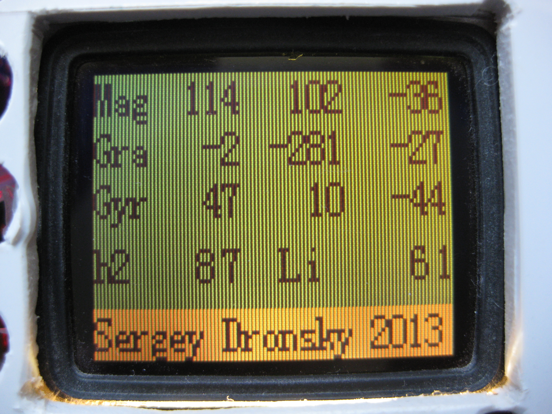
Screen 2:
From left to right, in rows:
Magnetic field sensor readings on three axes - X, Y, Z
The indications of the gravity sensor on the three axes - X, Y, Z The
indications of the acceleration field sensor on the three axes - X, Y, Z
The level of hydrogen, the illumination.
The last value in the first line is actually a deviation from the direction to the north magnetic pole.
Here is a curious picture:
As you can see, the compass needle and the face of the cube are almost parallel to each other and the direction to magnetic north.
Zero axis Z - because the sensor is installed vertically and the Z axis is horizontal, the Y axis is vertical.
Screen 3, temperature sensors:
A loop of five Dallas 18B20 sensors is connected to Cuba, the sketch at start determines the number of connected sensors and only polls them during further operation.
Here is a video of the launch of the sketch, which smoothly changes the brightness of each of their primary display colors at the start:
To be continued .
Source: https://habr.com/ru/post/243669/
All Articles