Likbez: image resize methods
Why an image scaled with bicubic interpolation does not look like in Photoshop. Why one program resizes quickly and the other does not, although the result is the same. Which resize method is better for increasing and which for reducing. What filters do and how do they differ.
In general, this was an introduction to another article, but it dragged on and turned into a separate material.

This person sits among the daisies to get your attention to the article.
')
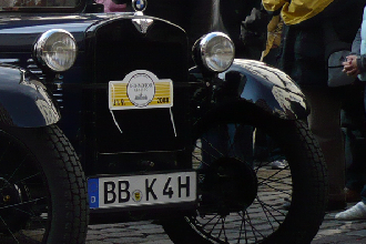
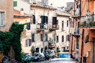
For visual comparison, I will use images of the same resolution of 1920 × 1280 ( one , the second ), which will result in sizes of 330 × 220, 1067 × 667 and 4800 × 3200. Under the illustrations it will be written how many milliseconds it took to resize this or that resolution. The numbers are given only to understand the complexity of the algorithm, so the specific hardware or software on which they are obtained is not so important.
This is the most primitive and fast method. For each pixel of the final image, one pixel of the source image is selected that is closest to its position, taking into account scaling. This method gives a pixelated image when zoomed in and a highly grainy image when zoomed out.

In general, the quality and performance of any reduction method can be estimated by the ratio of the number of pixels involved in the formation of the final image to the number of pixels in the original image. The greater this ratio, the more likely the algorithm is better and slower. A ratio equal to one means that at least each pixel of the original image has contributed to the final. But for advanced methods, it may be more than one. So here, if for example we reduce the image by the method of the nearest neighbor by 3 times on each side, then this ratio is 1/9. Those. most of the original pixels are not taken into account.


The theoretical speed depends only on the size of the final image. In practice, with a decrease, processor cache misses make a contribution: the smaller the scale, the less data is used from each line loaded into the cache.
The method is consciously used to reduce extremely rarely, because gives a very poor quality, although it can be useful with the increase. Because of the speed and ease of implementation, it is in all libraries and applications that work with graphics.
Affine transformations are a common method for image distortion. They allow you to rotate, stretch and reflect the image in one operation. Therefore, in many applications and libraries implementing the method of affine transformations, the function of changing images is simply a wrapper that calculates the coefficients for the transformation.
The principle of operation is that for each point of the final image a fixed set of points of the source is taken and interpolated in accordance with their mutual position and the selected filter. The number of points also depends on the filter. For bilinear interpolation, 2x2 source pixels are taken, for bicubic 4x4. This method gives a smooth image when zoomed in, but with a decrease the result is very similar to the nearest neighbor. See for yourself: theoretically, with a bicubic filter and a 3-fold decrease, the ratio of processed pixels to the original is 4² / 3² = 1.78. In practice, the result is much worse. in existing implementations, the filter window and the interpolation function are not scaled according to the image scale, and the pixels closer to the edge of the window are taken with negative coefficients (according to the function), i.e. do not make a useful contribution to the final image. As a result, the image reduced with the bicubic filter differs from the image reduced with the bilinear one, only in that it is even clearer. Well, for a bilinear filter and a reduction of three times the ratio of processed pixels to the original is 2² / 3² = 0.44, which is not fundamentally different from the nearest neighbor. In fact, affine transformations cannot be used to reduce more than 2 times. And even with a decrease to two times, they give noticeable ladder effects for lines.
Theoretically, there should be implementations of exactly affine transformations, scaling the filter window and the filter itself in accordance with the given distortions, but I have not seen such in popular open source libraries.


The running time is noticeably longer than that of the nearest neighbor, and depends on the size of the final image and the window size of the selected filter. From cache misses already almost does not depend, because source pixels are used at least two.
My humble opinion that using this method to arbitrarily reduce images is simply a bug , because the result is very bad and looks like the nearest neighbor, and you need much more resources for this method. However, this method has found wide application in programs and libraries. The most surprising is that this method is used in all browsers for the
In addition, this method is used by graphics cards for rendering three-dimensional scenes. But the difference is that the video cards for each texture prepare in advance a set of reduced versions (mip levels), and for the final rendering a level is selected with such a resolution that the texture reduction is no more than two times. In addition, to eliminate a sharp jump when changing a mip-level (when a textured object approaches or moves away), linear interpolation between adjacent mip-levels is used (this is already trilinear filtering). Thus, to draw each pixel of a three-dimensional object, it is necessary to interpolate between 2³ pixels. This gives a result that is acceptable for fast moving images in a time that is linear with respect to the final resolution.
With this method, the very mip-levels are created, with the help of it (if greatly simplified) full-screen anti-aliasing works in games. Its essence is in splitting the original image into a grid of final pixels and folding all the original pixels falling on each pixel of the final one in accordance with the area that falls under the final pixel. When using this method to increase, for each pixel of the final image there is exactly one pixel of the original. Therefore, the result to increase is equal to the nearest neighbor.


Two subspecies of this method can be distinguished: with the rounding of the borders of pixels to the nearest whole number of pixels and without. In the first case, the algorithm becomes unsuitable for scaling less than 3 times, because for any one final pixel there may be one source, and for the next one - four (2x2), which leads to imbalances at the local level. At the same time, the algorithm with rounding can obviously be used in cases when the size of the original image is a multiple of the size of the final image, or the reduction scale is rather small (the versions with a resolution of 330 × 220 are almost the same). The ratio of processed pixels to the original when rounding borders is always one.


The subspecies without rounding gives excellent quality while decreasing at any scale, and with increasing gives a strange effect when most of the original pixel on the final image looks homogeneous, but at the edges a transition is visible. The ratio of processed pixels to the original without the rounding of borders can be from one to four, because each source pixel contributes either to one final pixel, or to two adjacent ones, or to four neighboring pixels.


The performance of this method to reduce is lower than that of affine transformations, because all the pixels of the original are involved in the calculation of the final image. The version with rounding to the nearest borders is usually several times faster. It is also possible to create separate versions for scaling a fixed number of times (for example, a decrease of 2 times), which will be even faster.
This method is used in the
This method is similar to affine transformations in that filters are used, but it has not a fixed window, but a window proportional to the scale. For example, if the filter window size is 6, and the image size is reduced 2.5 times, then (2.5 * 6) ² = 225 pixels takes part in the formation of each pixel of the final image, which is much more than in the case of supersampling (from 9 to 16). Fortunately, convolutions can be considered in 2 passes, first in one direction, then in another, therefore the algorithmic complexity of calculating each pixel is not 225, but only (2.5 * 6) * 2 = 30. The contribution of each source pixel to the final one is times determined by the filter. The ratio of processed pixels to the original is entirely determined by the size of the filter window and is equal to its square. Those. for a bilinear filter, this ratio will be 4, for bicubic 16, for Lanczos 36. The algorithm works fine for both reduction and increase.


The speed of this method depends on all parameters: the size of the original image, the size of the final image, the size of the filter window.
This method is implemented in ImageMagick, GIMP, in the current version of Pillow with the ANTIALIAS flag.
One of the advantages of this method is that filters can be defined by a separate function that is not tied to the implementation of the method. At the same time, the function of the filter itself can be quite complex without much loss of performance, because the coefficients for all pixels in one column and for all pixels in one line are counted only once. Those. the filter function itself is called only (m + n) * w times, where m and n are the dimensions of the final image, and w is the size of the filter window. And to rivet these functions can be many, it would be a mathematical justification. In ImageMagick, for example, there are 15. Here’s what the most popular look like:
Bilinear filter (

Bicubic filter (

Lanczos filter

It is noteworthy that some filters have zones of negative coefficients (such as a bicubic filter or a Lanczos filter). This is necessary to make the transitions in the final image sharpen, which was the original.
In general, this was an introduction to another article, but it dragged on and turned into a separate material.
This person sits among the daisies to get your attention to the article.
')
For visual comparison, I will use images of the same resolution of 1920 × 1280 ( one , the second ), which will result in sizes of 330 × 220, 1067 × 667 and 4800 × 3200. Under the illustrations it will be written how many milliseconds it took to resize this or that resolution. The numbers are given only to understand the complexity of the algorithm, so the specific hardware or software on which they are obtained is not so important.
Nearest neighbor (Nearest neighbor)
This is the most primitive and fast method. For each pixel of the final image, one pixel of the source image is selected that is closest to its position, taking into account scaling. This method gives a pixelated image when zoomed in and a highly grainy image when zoomed out.
In general, the quality and performance of any reduction method can be estimated by the ratio of the number of pixels involved in the formation of the final image to the number of pixels in the original image. The greater this ratio, the more likely the algorithm is better and slower. A ratio equal to one means that at least each pixel of the original image has contributed to the final. But for advanced methods, it may be more than one. So here, if for example we reduce the image by the method of the nearest neighbor by 3 times on each side, then this ratio is 1/9. Those. most of the original pixels are not taken into account.
1920×1280 → 330×220 = 0,12 ms1920×1280 → 1067×667 = 1,86 ms1920×1280 → 4800×3200 = 22,5 msThe theoretical speed depends only on the size of the final image. In practice, with a decrease, processor cache misses make a contribution: the smaller the scale, the less data is used from each line loaded into the cache.
The method is consciously used to reduce extremely rarely, because gives a very poor quality, although it can be useful with the increase. Because of the speed and ease of implementation, it is in all libraries and applications that work with graphics.
Affine transformations
Affine transformations are a common method for image distortion. They allow you to rotate, stretch and reflect the image in one operation. Therefore, in many applications and libraries implementing the method of affine transformations, the function of changing images is simply a wrapper that calculates the coefficients for the transformation.
The principle of operation is that for each point of the final image a fixed set of points of the source is taken and interpolated in accordance with their mutual position and the selected filter. The number of points also depends on the filter. For bilinear interpolation, 2x2 source pixels are taken, for bicubic 4x4. This method gives a smooth image when zoomed in, but with a decrease the result is very similar to the nearest neighbor. See for yourself: theoretically, with a bicubic filter and a 3-fold decrease, the ratio of processed pixels to the original is 4² / 3² = 1.78. In practice, the result is much worse. in existing implementations, the filter window and the interpolation function are not scaled according to the image scale, and the pixels closer to the edge of the window are taken with negative coefficients (according to the function), i.e. do not make a useful contribution to the final image. As a result, the image reduced with the bicubic filter differs from the image reduced with the bilinear one, only in that it is even clearer. Well, for a bilinear filter and a reduction of three times the ratio of processed pixels to the original is 2² / 3² = 0.44, which is not fundamentally different from the nearest neighbor. In fact, affine transformations cannot be used to reduce more than 2 times. And even with a decrease to two times, they give noticeable ladder effects for lines.
Theoretically, there should be implementations of exactly affine transformations, scaling the filter window and the filter itself in accordance with the given distortions, but I have not seen such in popular open source libraries.
1920×1280 → 330×220 = 6.13 ms1920×1280 → 1067×667 = 17.7 ms1920×1280 → 4800×3200 = 869 msThe running time is noticeably longer than that of the nearest neighbor, and depends on the size of the final image and the window size of the selected filter. From cache misses already almost does not depend, because source pixels are used at least two.
My humble opinion that using this method to arbitrarily reduce images is simply a bug , because the result is very bad and looks like the nearest neighbor, and you need much more resources for this method. However, this method has found wide application in programs and libraries. The most surprising is that this method is used in all browsers for the
drawImage() canvas method (a visual example ), although for a simple display of pictures in an element, more accurate methods are used (except IE, it uses affine transformations for both cases). In addition, this method is used in OpenCV, the current version of the Python library Pillow (I hope to write about this separately) in Paint.NET.In addition, this method is used by graphics cards for rendering three-dimensional scenes. But the difference is that the video cards for each texture prepare in advance a set of reduced versions (mip levels), and for the final rendering a level is selected with such a resolution that the texture reduction is no more than two times. In addition, to eliminate a sharp jump when changing a mip-level (when a textured object approaches or moves away), linear interpolation between adjacent mip-levels is used (this is already trilinear filtering). Thus, to draw each pixel of a three-dimensional object, it is necessary to interpolate between 2³ pixels. This gives a result that is acceptable for fast moving images in a time that is linear with respect to the final resolution.
Supersampling
With this method, the very mip-levels are created, with the help of it (if greatly simplified) full-screen anti-aliasing works in games. Its essence is in splitting the original image into a grid of final pixels and folding all the original pixels falling on each pixel of the final one in accordance with the area that falls under the final pixel. When using this method to increase, for each pixel of the final image there is exactly one pixel of the original. Therefore, the result to increase is equal to the nearest neighbor.
Two subspecies of this method can be distinguished: with the rounding of the borders of pixels to the nearest whole number of pixels and without. In the first case, the algorithm becomes unsuitable for scaling less than 3 times, because for any one final pixel there may be one source, and for the next one - four (2x2), which leads to imbalances at the local level. At the same time, the algorithm with rounding can obviously be used in cases when the size of the original image is a multiple of the size of the final image, or the reduction scale is rather small (the versions with a resolution of 330 × 220 are almost the same). The ratio of processed pixels to the original when rounding borders is always one.
1920×1280 → 330×220 = 7 ms1920×1280 → 1067×667 = 15 ms1920×1280 → 4800×3200 = 22,5 msThe subspecies without rounding gives excellent quality while decreasing at any scale, and with increasing gives a strange effect when most of the original pixel on the final image looks homogeneous, but at the edges a transition is visible. The ratio of processed pixels to the original without the rounding of borders can be from one to four, because each source pixel contributes either to one final pixel, or to two adjacent ones, or to four neighboring pixels.
1920×1280 → 330×220 = 19 ms1920×1280 → 1067×667 = 45 ms1920×1280 → 4800×3200 = 112 msThe performance of this method to reduce is lower than that of affine transformations, because all the pixels of the original are involved in the calculation of the final image. The version with rounding to the nearest borders is usually several times faster. It is also possible to create separate versions for scaling a fixed number of times (for example, a decrease of 2 times), which will be even faster.
This method is used in the
gdImageCopyResampled() function of the GD library included in PHP in the OpenCV (INTER_AREA flag), Intel IPP, AMD Framewave. About the same principle works libjpeg, when it opens images in a reduced form several times. The latter allows many applications to open JPEG images in advance reduced several times without any special overhead (in practice, libjpeg opens thumbnails even a little faster than full-sized ones) and then apply other methods to resize to exact sizes. For example, if you want to regenerate JPEG with a resolution of 1920 × 1280 to a resolution of 330 × 220, you can open the original image at a resolution of 480 × 320 and then reduce it to the desired 330 × 220.Convolutions (Convolution)
This method is similar to affine transformations in that filters are used, but it has not a fixed window, but a window proportional to the scale. For example, if the filter window size is 6, and the image size is reduced 2.5 times, then (2.5 * 6) ² = 225 pixels takes part in the formation of each pixel of the final image, which is much more than in the case of supersampling (from 9 to 16). Fortunately, convolutions can be considered in 2 passes, first in one direction, then in another, therefore the algorithmic complexity of calculating each pixel is not 225, but only (2.5 * 6) * 2 = 30. The contribution of each source pixel to the final one is times determined by the filter. The ratio of processed pixels to the original is entirely determined by the size of the filter window and is equal to its square. Those. for a bilinear filter, this ratio will be 4, for bicubic 16, for Lanczos 36. The algorithm works fine for both reduction and increase.
1920×1280 → 330×220 = 76 ms1920×1280 → 1067×667 = 160 ms1920×1280 → 4800×3200 = 1540 msThe speed of this method depends on all parameters: the size of the original image, the size of the final image, the size of the filter window.
This method is implemented in ImageMagick, GIMP, in the current version of Pillow with the ANTIALIAS flag.
One of the advantages of this method is that filters can be defined by a separate function that is not tied to the implementation of the method. At the same time, the function of the filter itself can be quite complex without much loss of performance, because the coefficients for all pixels in one column and for all pixels in one line are counted only once. Those. the filter function itself is called only (m + n) * w times, where m and n are the dimensions of the final image, and w is the size of the filter window. And to rivet these functions can be many, it would be a mathematical justification. In ImageMagick, for example, there are 15. Here’s what the most popular look like:
Bilinear filter (
bilinear or triangle in ImageMagick)Bicubic filter (
bicubic , catrom in ImageMagick)Lanczos filter
It is noteworthy that some filters have zones of negative coefficients (such as a bicubic filter or a Lanczos filter). This is necessary to make the transitions in the final image sharpen, which was the original.
Source: https://habr.com/ru/post/243285/
All Articles