Oil Rows in R
“Price charts are great to predict the past”
Peter Lynch
I somehow could not deal with time series in practice. I, of course, read about them and had some idea in the course of the course on how the analysis is carried out in general, but it is well known that what is said in textbooks on statistics and machine learning does not always reflect the real state of affairs.
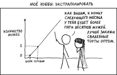
Probably, many are following with interest the pirouettes that the oil price curve makes. The schedule looks chaotic, too regular, and making some predictions on it is a very ungrateful task. Of course, you can bring down all the power of statistical, economic-mathematical and expert methods to the time series, but we will try to deal with technical analysis - of course, based on R.
When working with normal time series, you can use the standard approach:
')
There is a very convenient data source - Quandl ; it provides an interface for Matlab, Python, R. For R, just install one package:
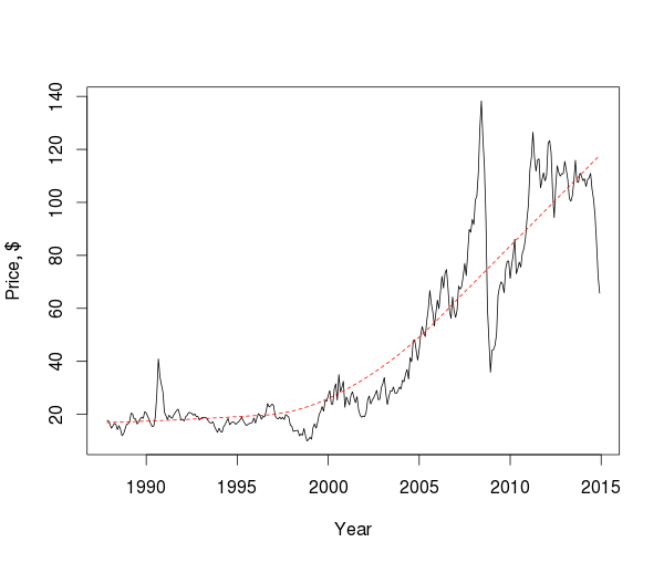
If we consider prices on the scale of decades, then we can see several peaks and falls and the direction of the trend, but in general it is difficult to draw any significant conclusions, so we examine the components of the series.
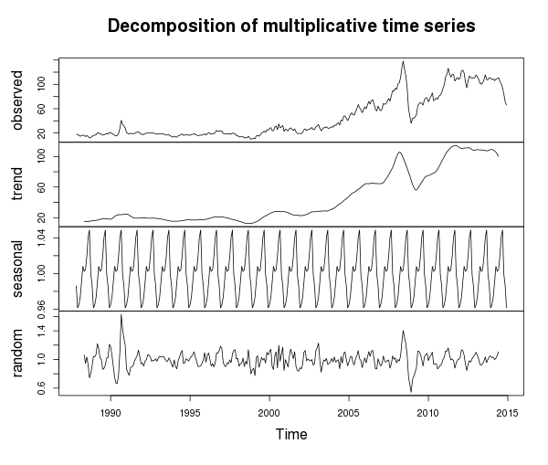
It seems that everything is clear with the trend - in the 21st century there is a steady upward trend until recently (with the exception of interesting years), a number of non - stationary - the Dicky-Fuller advanced test also proves this:
On the other hand, with a fairly high degree of confidence, it can be argued that the first-order differences of the series are stationary, i.e. This is an integrated first-order time series (this fact will further allow us to apply the Box-Jenkins methodology ).
In addition, it turns out that there is a seasonal component, which is difficult to see on the general chart. If you look closely, then besides the rather high volatility , you can see two price hikes during the year (which may be due to the increased consumption of oil in the winter period and the holiday season). On the other hand, there is a random component, the weight of which increases especially in critical years (for example, the 2008 financial crisis).
Sometimes it is preferable to work with data after a one-parameter Box-Cox transformation , which allows to stabilize the variance and bring the data to a more normal form:
As for the most slippery topic, namely, extrapolation, in the article “Crude Oil Price Forecasting Techniques: a Comprehensive Review of Literature” the authors note that, depending on the length of the time gap, the models are applicable:
After all the formalities, we will use the function
What worked out well on the top chart was retraining : the neural network caught the last pattern in the row and began to copy it. On the average chart, the network not only copies the last pattern, but also combines it well with the trend, which gives some realism to the forecast. In the lower graph it turned out ... some kind of unintelligible curve. Graphs well illustrate how predictions change depending on data smoothing. In any case, for products with high (for various reasons) volatility, predictions for such a time period cannot be trusted, so we will immediately move on to the short-term period, and at the same time compare several different models - ARIMA , tbats and neural network. We will use the data for the last half year and especially highlight the month of December in the series short.test - for testing purposes.
The neural network, having retrained, went somewhat into the astral, and ARIMA showed a very interesting relationship - interesting in terms of proximity to the real picture. Below is a comparison of the predictions of each model with real data in December and mean absolute percentage error :
I will not comment on long-term forecasts: it is obvious that they are already incorrect and incorrect in this situation. But ARIMA showed very good results for the short term. Also pay attention to the following facts. Oil prices dropped:
It kind of hints at us that the process of changing the price of oil is far from a process that is regulated by random parameters.
Peter Lynch
I somehow could not deal with time series in practice. I, of course, read about them and had some idea in the course of the course on how the analysis is carried out in general, but it is well known that what is said in textbooks on statistics and machine learning does not always reflect the real state of affairs.
Probably, many are following with interest the pirouettes that the oil price curve makes. The schedule looks chaotic, too regular, and making some predictions on it is a very ungrateful task. Of course, you can bring down all the power of statistical, economic-mathematical and expert methods to the time series, but we will try to deal with technical analysis - of course, based on R.
When working with normal time series, you can use the standard approach:
')
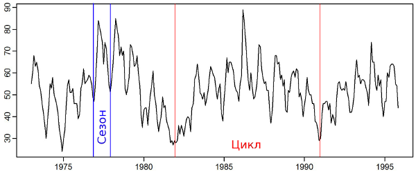
- Visual analysis
- Decomposition of a series and study of its component: seasonality, cyclicity, trend
- Building a mathematical model and forecasting
There is a very convenient data source - Quandl ; it provides an interface for Matlab, Python, R. For R, just install one package:
install.packages("Quandl") . I am interested in Europe Brent Crude Oil Spot Price - the spot price for Brent crude oil (below we use three sets of data in different details). library(Quandl) oil.ts <- Quandl("DOE/RBRTE", trim_start="1987-11-10", trim_end="2015-01-01", type="zoo") oil.tsw <-Quandl("DOE/RBRTE", trim_start="1987-11-10", trim_end="2015-01-01", type="zoo", collapse="weekly") oil.tsm <-Quandl("DOE/RBRTE", trim_start="1987-11-10", trim_end="2015-01-01", type="ts", collapse="monthly") plot(oil.tsm, xlab="Year", ylab="Price, $", type="l") lines(lowess(oil.tsm), col="red", lty="dashed") If we consider prices on the scale of decades, then we can see several peaks and falls and the direction of the trend, but in general it is difficult to draw any significant conclusions, so we examine the components of the series.
plot(decompose(oil.tsm, type="multiplicative")) It seems that everything is clear with the trend - in the 21st century there is a steady upward trend until recently (with the exception of interesting years), a number of non - stationary - the Dicky-Fuller advanced test also proves this:
>library(tseries) >library(forecast) >adf.test(oil.tsm, alternative=c('stationary')) Augmented Dickey-Fuller Test data: oil.tsm Dickey-Fuller = -2.7568, Lag order = 6, p-value = 0.2574 alternative hypothesis: stationary On the other hand, with a fairly high degree of confidence, it can be argued that the first-order differences of the series are stationary, i.e. This is an integrated first-order time series (this fact will further allow us to apply the Box-Jenkins methodology ).
>adf.test(diff(oil.tsm), alternative=c('stationary')) Augmented Dickey-Fuller Test data: diff(oil.tsm) Dickey-Fuller = -8.0377, Lag order = 6, p-value = 0.01 alternative hypothesis: stationary > ndiffs(oil.tsm) [1] 1 In addition, it turns out that there is a seasonal component, which is difficult to see on the general chart. If you look closely, then besides the rather high volatility , you can see two price hikes during the year (which may be due to the increased consumption of oil in the winter period and the holiday season). On the other hand, there is a random component, the weight of which increases especially in critical years (for example, the 2008 financial crisis).
Sometimes it is preferable to work with data after a one-parameter Box-Cox transformation , which allows to stabilize the variance and bring the data to a more normal form:
L <- BoxCox.lambda(ts(oil.ts, frequency=260), method="loglik") Lw <- BoxCox.lambda(ts(oil.tsw, frequency=52), method="loglik") Lm <- BoxCox.lambda(oil.tsm, method="loglik") As for the most slippery topic, namely, extrapolation, in the article “Crude Oil Price Forecasting Techniques: a Comprehensive Review of Literature” the authors note that, depending on the length of the time gap, the models are applicable:
- for the medium and long term, nonlinear models are more like - the same neural networks, support vector machines;
- for the short term, ARIMA often surpasses neural networks.
After all the formalities, we will use the function
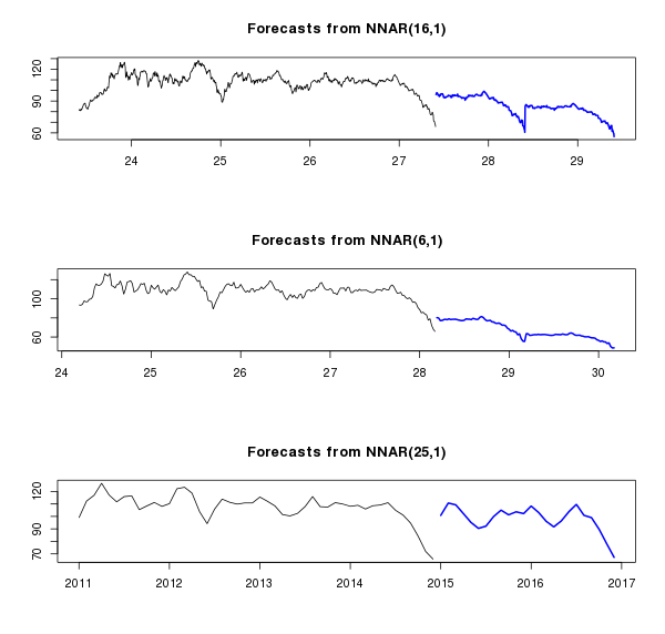
nnetar() that is present in the forecast package, with which it is possible to construct a neural network model of the series without any difficulties. At the same time we will do it for three rows - from more detailed (by day) to less detailed (by months). At the same time, let's see what will happen in the medium term - for example, over 2 years (in the graphs this is displayed in blue).Hidden text
# Fit NN for long-run fit.nn <- nnetar(ts(oil.ts, frequency=260), lambda=L, size=3) fcast.nn <- forecast(fit.nn, h=520, lambda=L) fit.nnw <- nnetar(ts(oil.tsw, frequency=52), lambda=Lw, size=3) fcast.nnw <- forecast(fit.nnw, h=104, lambda=Lw) fit.nnm <- nnetar(oil.tsm, lambda=Lm, size=3) fcast.nnm <- forecast(fit.nnm, h=24, lambda=Lm) par(mfrow=c(3, 1)) plot(fcast.nn, include=1040) plot(fcast.nnw, include=208) plot(fcast.nnm, include=48) What worked out well on the top chart was retraining : the neural network caught the last pattern in the row and began to copy it. On the average chart, the network not only copies the last pattern, but also combines it well with the trend, which gives some realism to the forecast. In the lower graph it turned out ... some kind of unintelligible curve. Graphs well illustrate how predictions change depending on data smoothing. In any case, for products with high (for various reasons) volatility, predictions for such a time period cannot be trusted, so we will immediately move on to the short-term period, and at the same time compare several different models - ARIMA , tbats and neural network. We will use the data for the last half year and especially highlight the month of December in the series short.test - for testing purposes.
Hidden text
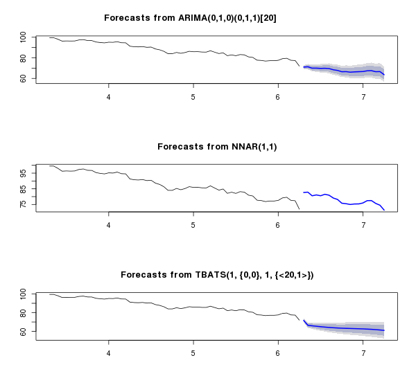
# Fit ARIMA, NN and ETS for short-run short <- ts(oil.ts[index(oil.ts) > "2014-06-30" & index(oil.ts) < "2014-12-01"], frequency=20) short.test <- as.numeric(oil.ts[index(oil.ts) >= "2014-12-01",]) h <- length(short.test) fit.arima <- auto.arima(short, lambda=L) fcast.arima <- forecast(fit.arima, h, lambda=L) fit.nn <- nnetar(short, size=7, lambda=L) fcast.nn <- forecast(fit.nn, h, lambda=L) fit.tbats <-tbats(short, lambda=L) fcast.tbats <- forecast(fit.tbats, h, lambda=L) par(mfrow=c(3, 1)) plot(fcast.arima, include=3*h) plot(fcast.nn, include=3*h) plot(fcast.tbats, include=3*h) 
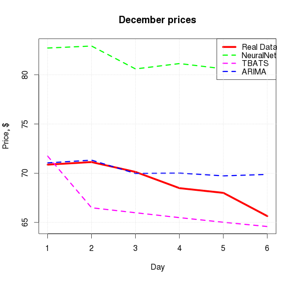
The neural network, having retrained, went somewhat into the astral, and ARIMA showed a very interesting relationship - interesting in terms of proximity to the real picture. Below is a comparison of the predictions of each model with real data in December and mean absolute percentage error :
Hidden text
par(mfrow=c(1, 1)) plot(short.test, type="l", col="red", lwd=5, xlab="Day", ylab="Price, $", main="December prices", ylim=c(min(short.test, fcast.arima$mean, fcast.tbats$mean, fcast.nn$mean), max(short.test, fcast.arima$mean, fcast.tbats$mean, fcast.nn$mean))) lines(as.numeric(fcast.nn$mean), col="green", lwd=3,lty=2) lines(as.numeric(fcast.tbats$mean), col="magenta", lwd=3,lty=2) lines(as.numeric(fcast.arima$mean), col="blue", lwd=3, lty=2) legend("topright", legend=c("Real Data","NeuralNet","TBATS", "ARIMA"), col=c("red","green", "magenta","blue"), lty=c(1,2,2,2), lwd=c(5,3,3,3)) grid() Hidden text
mape <- function(r, f){ len <- length(r) return(sum( abs(r - f$mean[1:len]) / r) / len * 100) } mape(short.test, fcast.arima) mape(short.test, fcast.nn) mape(short.test, fcast.tbats) | ARIMA | Nnet | Tbats |
| 1.99% | 18.26% | 4.00% |
Instead of conclusion
I will not comment on long-term forecasts: it is obvious that they are already incorrect and incorrect in this situation. But ARIMA showed very good results for the short term. Also pay attention to the following facts. Oil prices dropped:
- in September by 5%;
- in October - by 10%;
- in November - by 15%;
- for December ...?
It kind of hints at us that the process of changing the price of oil is far from a process that is regulated by random parameters.
Source: https://habr.com/ru/post/243211/
All Articles