Software renderer - 1: materiel
Software rendering is software image creation without the help of a GPU. This process can go in one of two modes: in real time (calculation of a large number of frames per second — necessary for interactive applications, for example, games) and in offline mode (at which the time that can be spent on calculating one frame, not so strictly limited - calculations can take hours or even days). I will only consider the real-time rendering mode.
This approach has both disadvantages and advantages. The obvious disadvantage is the performance - the CPU is not able to compete with modern video cards in this area. The advantages should be attributed to the independence of the video card - that is why it is used as a replacement for hardware rendering in cases where the video card does not support this or that feature (the so-called software fallback). There are also projects whose purpose is to completely replace hardware rendering with software, for example, WARP, which is part of Direct3D 11.
But the main advantage is the possibility of writing such a renderer independently. It serves educational purposes and, in my opinion, it is the best way to understand the underlying algorithms and principles.
')
This is exactly what will be discussed in a series of these articles. We will start with the ability to paint a pixel in a window with a specified color and build on it the ability to render a three-dimensional scene in real time, with moving textured models and lighting, as well as with the ability to move around this scene.
But in order to display at least the first polygon, it is necessary to master the mathematics on which it is built. The first part will be dedicated to her, so there will be many different matrices and other geometry in it.
At the end of the article there will be a link to the githab project, which can be considered as an example of implementation.
Despite the fact that the article will describe the very basics, the reader still needs a certain foundation for its understanding. This foundation: the basics of trigonometry and geometry, an understanding of Cartesian coordinate systems and basic operations on vectors. Also, it would be a good idea to read an article about the basics of linear algebra for game developers (for example, this one ), since I will skip the descriptions of some operations and dwell only on the most important ones from my point of view. I will try to show with the help of which some important formulas are drawn, but I will not describe them in detail - you can make full proofs yourself or find them in the relevant literature. In the course of the article, I will first try to give algebraic definitions of a particular concept, and then describe their geometric interpretation. Most of the examples will be in two-dimensional space, since my skills in drawing three-dimensional and, even more so, four-dimensional spaces leave much to be desired. Nevertheless, all examples are easily generalized to spaces of other dimensions. All articles will be more focused on the description of algorithms, rather than on their implementation in the code.
Vector - one of the key concepts in three-dimensional graphics. And although linear algebra gives it a very abstract definition, in the framework of our tasks, under the n- dimensional vector, we can simply understand an array of n real numbers: an element of the space R n :
The interpretation of these numbers depends on the context. The two most frequent: these numbers specify the coordinates of a point in space or a directional displacement. Despite the fact that their representation is the same ( n real numbers), their concepts are different - the point describes the position in the coordinate system, and the displacement does not have a position as such. In the future, we can also determine the point using the offset, implying that the offset occurs from the origin.
As a rule, in the majority of game and graphic engines there is a class of a vector just like a set of numbers. The meaning of these numbers depends on the context in which they are used. In this class, methods are defined both for working with geometric vectors (for example, calculating the vector product) and with points (for example, calculating the distance between two points).
In order to avoid confusion, within the framework of the article we will no longer understand the abstract set of numbers by the word "vector", but we will call so the offset.
The only operation on vectors that I want to dwell on in detail (because of its fundamental nature) is a scalar product. As the name implies, the result of this work is a scalar, and it is determined by the following formula:

The dot product has two important geometric interpretations.
This section is intended to prepare the basis for the introduction of matrices. I, using the example of the world and local systems, will show for what reasons several coordinate systems are used, rather than one, and how to describe one coordinate system relative to another.
Imagine that we needed to draw a scene with two models, for example:
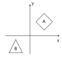
What coordinate systems naturally follow from such a statement? The first is the coordinate system of the scene itself (which is shown in the figure). This is a coordinate system describing the world that we are going to draw - this is why it is called “world” (in the pictures it will be marked with the word “world”). She "binds" all the objects of the scene together. For example, the coordinates of the center of the object A in this coordinate system are (1, 1) , and the coordinates of the center of the object B are (-1, -1) .
Thus, one coordinate system is already there. Now we need to think about the way in which models come to us, which we will use in the scene.
For simplicity, we assume that the model is described simply as a list of points (“vertices”) of which it consists. For example, model B consists of three points that come to us in the following format:
v 0 = (x 0 , y 0 )
v 1 = (x 1 , y 1 )
v 2 = (x 2 , y 2 )
At first glance, it would be great if they were already described in the “world” system we need! Imagine, you are adding a model to the stage, and it is already where we need it. For model B, it might look like this:
v 0 = (-1.5, -1.5)
v 1 = (-1.0, -0.5)
v 2 = (-0.5, -1.5)
But to use this approach will not work. There is an important reason for this: it makes it impossible to use the same model again in different scenes. Imagine that you were given model B , which was modeled in such a way that when you add it to the stage, it appears in the right place for us, as in the example above. Then, suddenly, the demand has changed - we want to move it to a completely different position. It turns out that the person who created this model will have to move it independently and then give it back to you. Of course, this is complete absurdity. An even stronger argument is that in the case of interactive applications, the model can move, rotate, animate on the stage - what can an artist do a model in all possible positions? That sounds even more stupid.
The solution to this problem is the “local” coordinate system of the model. We model the object in such a way that its center (or that which can be conventionally taken as such) is located at the origin. Then we programmatically orient (move, rotate, etc.) the local coordinate system of the object to the position we need in the world system. Returning to the scene above, object A (unit square, rotated 45 degrees clockwise) can be modeled as follows:

The description of the model in this case will look as follows:
v 0 = (-0.5, 0.5)
v 1 = (0.5, 0.5)
v 2 = (0.5, -0.5)
v 3 = (-0.5, -0.5)
And, accordingly, the position in the scene of two coordinate systems - the world and local object A :

This is one example of why having multiple coordinate systems makes life easier for developers (and artists!). There is another reason - the transition to a different coordinate system can simplify the necessary calculations.
There is no such thing as "absolute coordinates". A description of something always happens relative to some kind of coordinate system. Including the description of another coordinate system.
We can build a peculiar hierarchy of coordinate systems in the example above:
In our case, this hierarchy is very simple, but in real situations it can have much stronger branching. For example, a local coordinate system of an object may have child systems that are responsible for the position of one or another part of the body.
Each child coordinate system can be described relative to the parent using the following values:
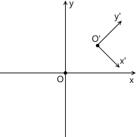
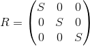
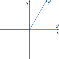
For example, in the picture below, the origin of the system x'y ' (denoted as O' ) is located at (1, 1) , and the coordinates of its base vectors i ' and j' are (0.7, -0.7) and (0.7, 0.7 ) respectively (which roughly corresponds to the axes rotated 45 degrees clockwise).
We do not need to describe the world coordinate system relative to any other, because the world system is the root of the hierarchy, we do not care where it is located or how it is oriented. Therefore, to describe it, we use the standard basis:
The coordinates of the point P in the parent coordinate system (denoted by P parent ) can be calculated using the coordinates of this point in the child system (denoted as P child ) and the orientation of this child system relative to the parent (described using the origin O and the base vectors i ' and j ' ) as follows:

Let's go back to the example scene above. We orient the local coordinate system of object A relative to the world:
As we already know, in the process of drawing we will need to transfer the coordinates of the vertices of the object from the local coordinate system to the world one. For this we need a description of the local coordinate system relative to the world. It looks like this: the origin is at the point (1, 1) , and the coordinates of the basis vectors are (0.7, -0.7) and (0.7, 0.7) (the method of calculating the coordinates of the basis vectors after the rotation will be described later, so far we have enough result) .
For example, take the first vertex v = (-0.5, 0.5) and calculate its coordinates in the world system:
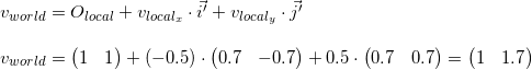
The fidelity of the result can be seen by looking at the image above.
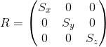
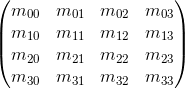
The matrix of dimension mxn is the corresponding dimension table of numbers. If the number of columns in the matrix is equal to the number of rows, then the matrix is called square. For example, a 3 x 3 matrix looks like this:

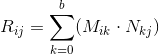
Suppose we have two matrices: M (dimension axb ) and N (dimension cxd ). The expression R = M · N is defined only if the number of columns in the matrix M is equal to the number of rows in the matrix N (that is, b = c ). The dimension of the resulting matrix will be equal to axd (i.e., the number of rows is equal to the number of rows M and the number of columns is the number of columns in N ), and the value located at position ij is calculated as the scalar product of the i -th row M by the jth column n :
If the result of multiplying two matrices M · N is defined, then this does not mean that the multiplication in the opposite direction is also determined - N · M (the number of rows and columns may not coincide). In the general case, the operation of matrix multiplication is also not commutative: M · N ≠ N · M.
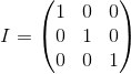
A unit matrix is a matrix that does not change another matrix multiplied by it (ie, M · I = M ) - a kind of analogue of one for ordinary numbers:
We can also represent a vector as a matrix. There are two possible ways to do this, which are called “row vector” and column vector “”. As the name implies, a row vector is a vector represented as a matrix with one row, and a column vector is a vector represented as a matrix with one column.
Row Vector:
Column Vector:

Further, we will often come across the operation of multiplying the matrix by a vector (which will be explained in the next section), and, running ahead, the matrices with which we will work will have the dimension of either 3 x 3 or 4 x 4 .
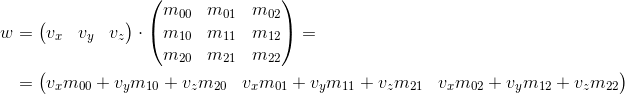
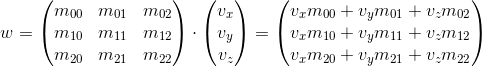
Consider how we can multiply the three-dimensional vector by a 3 x 3 matrix (similar arguments apply for other dimensions). By definition, two matrices can be multiplied if the number of columns in the first matrix equals the number of rows in the second. Thus, since we can represent a vector both as a 1 x 3 matrix (row vector) and as a 3 x 1 matrix (column vector), we get two possible options:
As you can see, we get a different result in each case. This can lead to random errors if the API allows you to multiply a vector by a matrix on both sides, because, as we will see later, the transformation matrix implies that the vector will be multiplied by one of two methods. So, in my opinion, the API is better to stick with only one of two options. Within these articles I will use the first option - i.e. the vector is multiplied by the matrix on the left. If you decide to use a different order, then, in order to get correct results, you will need to transpose all the matrices that will later be found in this article, and replace the word “row” with a “column”. It also affects the order of matrix multiplication in the presence of several transformations (it will be discussed in more detail later).
It is also seen from the result of the multiplication that the matrix in a certain way (depending on the value of its elements) changes the vector that was multiplied by it. It can be such transformations as rotation, scaling and others.
Another very important property of the matrix multiplication operation, which will be useful to us later, is distributivity with respect to addition:

As we saw in the previous section, the matrix in a certain way transforms the vector multiplied by it.
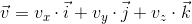
Once again, remember that any vector can be represented as a linear combination of basis vectors:

Multiply this expression by the matrix:

Using distributivity with respect to addition, we get:

We have already seen this before, when we considered how to transfer the coordinates of a point from the child system to the parent system, then it looked like this (for three-dimensional space):

There are two differences between these two expressions - in the first expression there is no movement ( O child , we will consider this moment in more detail when we talk about linear and affine transformations), and the vectors i ' , j' and k 'are replaced by iM , jM and kM respectively. Consequently, iM , jM and kM are the basis vectors of the child coordinate system and we transfer the point v child (v x , v y , v y ) from this child coordinate system to the parent ( v transformed = v parent M ).
The transformation process can be depicted as follows using the counterclockwise rotation as an example ( xy is the original, parental coordinate system, x'y ' is a daughter one resulting from the transformation):
Just in case, to make sure that we understand the meaning of each of the vectors used above, we list them again:
Now consider what happens when you multiply the basis vectors by the matrix M :

It can be seen that the basis vectors of the new child coordinate system obtained as a result of multiplication by the matrix M coincide with the rows of the matrix. This is the very geometric interpretation we were looking for.Now, having seen the transformation matrix, we will know where to look, in order to understand what it is doing - it is enough to present its rows as basis vectors of the new coordinate system. The transformation that occurs with the coordinate system will be the same as the transformation that occurs with the vector multiplied by this matrix.
We can also combine transformations presented in the form of matrices by multiplying them by each other:

Thus, matrices are a very convenient tool for describing and combining transformations.
To begin, consider the most commonly used linear transformations. Linear transformation is a transformation that satisfies two properties:
An important consequence is that a linear transformation cannot contain displacements (this is also the reason why the O child term was absent in the previous section) because, according to the second formula, 0 is always displayed as 0 .
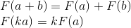
Consider rotation in two-dimensional space. This is a transformation that rotates the coordinate system at a given angle. As we already know, it is enough for us to calculate the new coordinate axes (obtained after rotation at a given angle), and use them as rows of the transformation matrix. The result is easily obtained from the basic geometry:

Example:

The result for rotation in three-dimensional space is obtained in a similar way, with the only difference that we rotate the plane composed of two coordinate axes, and fix the third (around which rotation takes place). For example, the rotation matrix around the x axis looks like this:

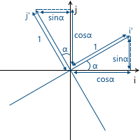
We can change the scale of the object with respect to all axes using the following matrix: The
axes of the transformed coordinate system will be directed the same way as the original coordinate system, but will require S times the length for one unit of measurement:
Example:
Scaling with the same ratio relative to all axes is called uniform. But we can also scale with different coefficients along different (nonuniform) axes:
As the name implies, this transformation shifts along the coordinate axis, leaving the remaining axes intact:
Accordingly, the y- axis shift matrix is as follows:

Example:

The matrix for the three-dimensional space is constructed in a similar way. For example, the option for shifting the x axis :

Although this transformation is used very rarely, it will be useful to us in the future when we consider affine transformations.
There is already a decent number of transformations in our stock, which can be represented as a 3 x 3 matrix, but we lack one more — displacement. Unfortunately, it is impossible to express displacement in three-dimensional space using 3 x 3 matrices, since displacement is not a linear transformation. The solution to this problem is homogeneous coordinates, which we will consider later.
Our final goal is to draw a three-dimensional scene on a two-dimensional screen. Thus, we need to project our stage onto a plane in one way or another. There are two most commonly used types of projections - orthographic and central (another name is perspective).
When the human eye looks at the three-dimensional scene, the objects that are farther from it become smaller in the final image, which the person sees - this effect is called perspective. The orthographic projection ignores the perspective, which is a useful feature when working in various CAD systems (as well as in 2D games). The central projection has this property and therefore adds a significant proportion of realism. In this article we will consider only her.
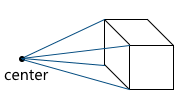
Unlike the orthographic projection, the lines in the perspective projection are not parallel to each other, but intersect at a point called the center of the projection. The center of the projection is the “eye” with which we look at the scene — the virtual camera:
The image is formed on a plane located at a given distance from the virtual camera. Accordingly, the greater the distance from the camera, the larger the projection size:

Consider the simplest example: the camera is located at the origin of coordinates, and the projection plane is at a distance d from the camera. We know the coordinates of the point we want to project: (x, y, z) . Find the coordinate x p of the projection of this point on the plane:
This picture shows two similar triangles - CDP and CBA (at three angles):
Accordingly, the relationship between the parties remains:
We get the result for the x coordinates:

And, similarly, for the y coordinates:

Later, we will need to use this transformation to form projected image. And here a problem arises - we cannot imagine dividing by z- coordinate in three-dimensional space using a matrix. The solution to this problem, as well as in the case of the displacement matrix, are homogeneous coordinates.
To date, we are faced with two problems:
Both of these problems solves the use of uniform coordinates. Homogeneous coordinates - a concept from projective geometry. Projective geometry studies projective spaces, and, in order to understand the geometric interpretation of homogeneous coordinates, it is necessary to get to know them.
Below we will consider definitions for two-dimensional projective spaces, since they are easier to portray. Similar reasoning applies to three-dimensional projective spaces (we will use them in the future).
We define a ray in R 3 as follows: a ray is a set of vectors of the form kv ( k is a scalar, v is a non-zero vector, an element of R 3 ). Those.the vector v defines the direction of the ray:

Now we can proceed to the definition of the projective space. The projective plane (i.e., a projective space with a dimension equal to two) P 2 , associated with the space R 3 , is the set of rays in R 3 . Thus, the “point” in P 2 is a ray in R 3 .
Accordingly, two vectors in R 3 set the same element in P 2 , if one of them can be obtained by multiplying the second by a scalar (since in this case they lie on the same ray):

For example, the vectors (1, 1, 1) and (5, 5, 5) represent the same ray, and therefore are the same “point” in the projective plane.
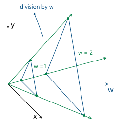
So we came to homogeneous coordinates. Each element in the projective plane is defined by a ray of three coordinates (x, y, w) (the last coordinate is called w instead of z — the generally accepted convention) —the coordinates are called homogeneous and are determined with an accuracy to a scalar. This means that we can multiply (or divide) homogeneous coordinates by a scalar, and they will still represent the same “point” in the projective plane.
In the following, we will use homogeneous coordinates to represent affine (containing displacement) transformations and projections. But before that, one more question needs to be solved: how to represent in the form of homogeneous coordinates the vertices of the model already given to us? Since the “addition” to the homogeneous coordinates occurs due to the addition of the third coordinate w , the question boils down to what value of w we need to use. The answer to this question is any non-zero. The difference in the use of different values of w is the convenience of working with them.
And, as will be understood later (and partly clear intuitively), the most convenient value of w is one. The advantages of this choice are as follows:
Thus, we choose the value w = 1 , which means that our input data in homogeneous coordinates will now look like this (of course, we’ve already added one, and will not be in the model description itself):
v 0 = (x 0 , y 0 , 1)
v 1 = (x 1 , y 1 , 1)
v 2 = (x 2 , y 2 , 1)
Now we need to consider a special case when working with the w- coordinate. Namely - its equality to zero. Above we said that we can choose any value of w, not equal to zero, for expansion to homogeneous coordinates. We cannot take w = 0 , in particular, because it will not allow moving this point (since, as we will see later, the movement occurs precisely due to the value in the w coordinate). Also, if the w coordinate of the point is zero, we can consider it as a point "at infinity", because when we try to return to the plane w = 1, we get the division by zero:
And, although we cannot use the zero value for the model vertices, we can use it for vectors! This will lead to the fact that the vector will not be subject to movement during transformations - which makes sense, because the vector does not describe the position. For example, when transforming the normal, we cannot move it, otherwise we will get an incorrect result. We will take a closer look at this when the need arises to transform vectors.
In this connection, it is often written that for w = 1 we describe a point, and for w = 0 , a vector.
As I already wrote, we used the example of two-dimensional projective projective spaces, but in fact we will use three-dimensional projective spaces, which means each point will be described by 4 coordinates: (x, y, z, w) .
Now we have all the necessary tools to describe affine transformations. Affine transformations are linear transformations with subsequent displacement. They can be described as follows:

We can also use 4 x 4 matrices to describe affine transformations using homogeneous coordinates:
Consider the result of multiplying the vector, represented as homogeneous coordinates, and multiplying by 4 x 4 matrix:
As you can see, the difference from the transformation , represented in the form of a 3 x 3 matrix, consists in the presence of the 4th coordinate, as well as the new terms in each of the coordinates of the form v w · m 3i . Using this, and implying w = 1, we can imagine the movement as follows:
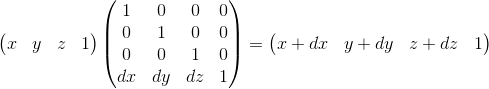
Here you can make sure that the choice of w = 1 is correct . To represent the displacement dx, we use a term of the form w · dx / w . Accordingly, the last row of the matrix looks like (dx / w, dy / w, dz / w, 1) . In the case of w = 1, we can simply omit the denominator.
This matrix also has a geometric interpretation. Recall the shift matrix, which we considered earlier. It has exactly the same format, the only difference is that the fourth axis is shifted, thus shifting the three-dimensional subspace located in the hyperplane w = 1 by the corresponding values.
A virtual camera is the “eye” with which we look at the scene. Before proceeding further, it is necessary to understand how to describe the position of the camera in space, and what parameters are necessary for the formation of the final image.
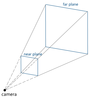
The camera parameters set the truncated view pyramid (view frustum), which determines which part of the scene falls into the final image:
Consider them in turn:
We can move and rotate the camera, changing the position and orientation of its coordinate system. Code example:
Now we have all the necessary foundation in order to describe by steps the steps that are necessary to obtain an image of a three-dimensional scene on a computer screen. For simplicity, we will assume that the pipeline draws one object at a time.
Incoming parameters of the pipeline:
At this stage, we transform the object vertices from the local coordinate system into the world one.
Suppose that the orientation of an object in the world coordinate system is defined by the following parameters:
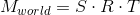
We call the matrices of these transformations T , R, and S, respectively. To obtain the final matrix, which will transform an object into a world coordinate system, we need only to multiply them. It is important to note here that the order of multiplication of matrices plays a role - this directly follows from the fact that the multiplication of matrices is noncommutative.
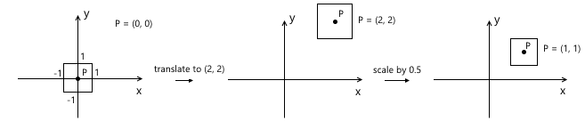
Recall that scaling occurs relative to the origin. If we first displace the object to the desired point, and then apply a scale to it, we will get the wrong result - the position of the object will change again after scaling. A simple example:
A similar rule applies with respect to rotation - it occurs relative to the origin, which means that the position of the object will change if we first make a movement.
Thus, the correct sequence in our case is as follows: scaling - rotation - offset:
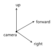
The transition to the camera's coordinate system, in particular, is used to simplify further calculations. In this coordinate system, the camera is located at the origin, and its axes are the forward , right , up vectors, which we considered in the previous section.
The transition to the camera coordinate system consists of two steps:
The first step can be easily represented as a matrix of displacement on (-pos x , -pos y , -pos z ) , where pos is the position of the camera in the world coordinate system:

To implement the second item, we use the property of the scalar product, which we considered at the very beginning - the scalar product calculates the length of the projection along a given axis. Thus, in order to transfer point A to the camera's coordinate system (taking into account the fact that the camera is at the origin, we did this in the first paragraph), we just need to take its scalar product with the vectors right , up , forward . Denote a point in the world coordinate system v , and the same point translated into the camera coordinate system, v ' , then:
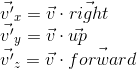
This operation can be represented as a matrix:
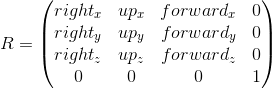
Combining these two transformations, we get the transition matrix to the camera coordinate system:

Schematically, this process can be depicted as follows:

As a result of the previous point, we obtained the coordinates of the object's vertices in the camera's coordinate system. The next thing to do is to make a projection of these vertices on the plane and “cut off” the extra vertices. The vertex of the object is cut off if it lies outside the pyramid of the review (i.e. its projection does not lie on that part of the plane which the pyramid of the survey covers). For example, vertex v 1 in the figure below:

Both of these tasks are partially solved by the projection matrix. “Partially” - because it does not produce the projection itself, but prepares the w- coordinate of the vertex for this. Because of this, the name “projection matrix” does not sound very appropriate (although this is a fairly common term), and I will call it the clip matrix in the future, since it also displays the truncated view pyramid in a uniform clipping space (homogeneous clip space).
But first things first. So, the first is preparation for the projection. For this, we put the z- coordinate of the vertex in its w- coordinate. The projection itself (that is, division by z ) will occur upon further normalization of the w-coordinate — that is, when returning to the space w = 1 .
The next thing this matrix has to do is translate the coordinates of the vertices of the object from the camera space into a homogeneous clip space. This space, the coordinates of the non-clipped vertices in which are such that after applying the projection (i.e., dividing by the w- coordinate, since we saved the old z- coordinate in it), the coordinates of the vertex are normalized; satisfy the following conditions:

Inequality for z coordinates can vary for different APIs. For example, in OpenGL, it corresponds to what is above. In Direct3D, the z coordinate is displayed in the interval [0, 1] . We will use the OpenGL interval, i.e. [-1, 1] .
Such coordinates are called normalized device coordinates (normalized device coordinates or simply NDC).
Since we obtain the NDC coordinates by dividing the coordinates by w , the vertices in the cut-off space satisfy the following conditions:

Thus, by transferring the vertices to this space, we can find out whether it is necessary to cut the vertex simply by checking its coordinates for the inequalities above. Any vertex that does not satisfy these conditions must be cut off. The cut-off itself is a topic for a separate article, because its correct implementation leads to the creation of new vertices. So far, as a quick fix, we will not draw a face if at least one of its vertices is clipped. Of course, the result will not be very neat. For example, for a car model, it looks like this:
Total, this stage consists of the following steps:
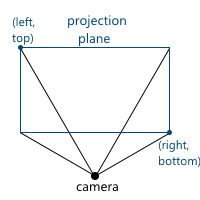
Now consider how we map the coordinates from the camera space to the clipping space. Recall that we decided to use the projection plane z = 1 . First we need to find a function that displays the coordinates lying on the intersection of the pyramid of the review and the projection plane in the interval [-1, 1] . For this we find the coordinates of the points defining this part of the plane. These two points have coordinates (left, top) and (right, bottom) . We will consider only the case when the pyramid of view is symmetrical about the direction of the camera.
We can calculate them using viewing angles:
We get:

Similarly for top and bottom :
Thus, we need to display the interval [left, right] , [bottom, top] , [near, far] in [-1; 1] . Find a linear function that gives this result for left and right :

Similarly, the function for the bottom and top is obtained:
The expression for z is different. Instead of considering a function of the form az + b, we will consider the function a · 1 / z + b , because later, when we implement the depth buffer, we will need to linearly interpolate the inverse of the z-coordinate. We will not consider this issue now, and just take it for this. We get:
Thus, we can write that the normalized coordinates are obtained as follows from the coordinates in the camera space:
We cannot immediately apply these formulas, because division by z will occur later, with normalization of w- coordinates. We can use this, and instead calculate the following values (multiplying by z), which after dividing by w , will result in normalized coordinates:
It is by these formulas that we transform into the cut-off space. We can write this transformation in matrix form (remembering additionally that we put z in the w coordinate):

To the current stage, we have the coordinates of the object vertices in the NDC. We need to translate them into screen coordinate system. Recall that the upper left corner of the projection plane was mapped to (-1, 1), and the lower right to (1, -1). For the screen, I will use the upper left corner as the origin of the coordinate system, with the axes pointing right and down:

This viewport transformation can be made using simple formulas:
Or, in matrix form:
We will leave using z ndc until the implementation of the depth buffer.
As a result, we have the coordinates of the vertices on the screen, which we use for drawing.
Below is an example of code that implements a pipeline using the method described above and performing drawing in wireframe mode (i.e., simply connecting vertices with lines). It also implies that the object is described by a set of vertices and a set of indexes of the vertices (faces) of which its polygons consist:
In this section, I will briefly explain how SDL2 can be used to implement rendering.
The first is, of course, the initialization of the library and the creation of the window. If only graphics are needed from SDL, then you can initialize with the SDL_INIT_VIDEO flag:
Then, create a texture into which we will render. I will use the ARGB8888 format, which means that each pixel in the texture will be allocated 4 bytes - three bytes on the RGB channels, and one on the alpha channel.
You need to remember to “clear” the SDL and all variables taken from it when the application exits:
We can use SDL_UpdateTexture to update the texture, which we will then display on the screen. This function accepts, among others, the following parameters:
It is logical to allocate the drawing functionality to the texture, represented by an array of bytes, in a separate class. It will allocate memory for the array, clear the texture, draw pixels and lines. Drawing a pixel can be done as follows (the order of bytes differs depending on SDL_BYTEORDER ):
Line drawing can be implemented, for example, by the Brezenham algorithm .
After using SDL_UpdateTexture , you must copy the texture into SDL_Renderer and display it on the screen using SDL_RenderPresent . Together:
That's all. Link to the project: https://github.com/loreglean/lantern .
This approach has both disadvantages and advantages. The obvious disadvantage is the performance - the CPU is not able to compete with modern video cards in this area. The advantages should be attributed to the independence of the video card - that is why it is used as a replacement for hardware rendering in cases where the video card does not support this or that feature (the so-called software fallback). There are also projects whose purpose is to completely replace hardware rendering with software, for example, WARP, which is part of Direct3D 11.
But the main advantage is the possibility of writing such a renderer independently. It serves educational purposes and, in my opinion, it is the best way to understand the underlying algorithms and principles.
')
This is exactly what will be discussed in a series of these articles. We will start with the ability to paint a pixel in a window with a specified color and build on it the ability to render a three-dimensional scene in real time, with moving textured models and lighting, as well as with the ability to move around this scene.
But in order to display at least the first polygon, it is necessary to master the mathematics on which it is built. The first part will be dedicated to her, so there will be many different matrices and other geometry in it.
At the end of the article there will be a link to the githab project, which can be considered as an example of implementation.
Despite the fact that the article will describe the very basics, the reader still needs a certain foundation for its understanding. This foundation: the basics of trigonometry and geometry, an understanding of Cartesian coordinate systems and basic operations on vectors. Also, it would be a good idea to read an article about the basics of linear algebra for game developers (for example, this one ), since I will skip the descriptions of some operations and dwell only on the most important ones from my point of view. I will try to show with the help of which some important formulas are drawn, but I will not describe them in detail - you can make full proofs yourself or find them in the relevant literature. In the course of the article, I will first try to give algebraic definitions of a particular concept, and then describe their geometric interpretation. Most of the examples will be in two-dimensional space, since my skills in drawing three-dimensional and, even more so, four-dimensional spaces leave much to be desired. Nevertheless, all examples are easily generalized to spaces of other dimensions. All articles will be more focused on the description of algorithms, rather than on their implementation in the code.
Vectors
Vector - one of the key concepts in three-dimensional graphics. And although linear algebra gives it a very abstract definition, in the framework of our tasks, under the n- dimensional vector, we can simply understand an array of n real numbers: an element of the space R n :
The interpretation of these numbers depends on the context. The two most frequent: these numbers specify the coordinates of a point in space or a directional displacement. Despite the fact that their representation is the same ( n real numbers), their concepts are different - the point describes the position in the coordinate system, and the displacement does not have a position as such. In the future, we can also determine the point using the offset, implying that the offset occurs from the origin.
As a rule, in the majority of game and graphic engines there is a class of a vector just like a set of numbers. The meaning of these numbers depends on the context in which they are used. In this class, methods are defined both for working with geometric vectors (for example, calculating the vector product) and with points (for example, calculating the distance between two points).
In order to avoid confusion, within the framework of the article we will no longer understand the abstract set of numbers by the word "vector", but we will call so the offset.
Scalar product
The only operation on vectors that I want to dwell on in detail (because of its fundamental nature) is a scalar product. As the name implies, the result of this work is a scalar, and it is determined by the following formula:
The dot product has two important geometric interpretations.
- Measure the angle between vectors.
Consider the following triangle derived from three vectors:
Writing for him the cosine theorem and reducing the expression, we come to the record:
Since, by definition, the length of a nonzero vector is greater than 0, the cosine of an angle determines the sign of the scalar product and its equality to zero. We get (assuming that the angle is from 0 to 360 degrees):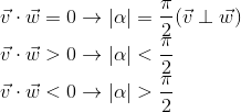
- The dot product calculates the length of the projection of the vector on the vector.
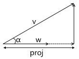
From the definition of the cosine of an angle we get: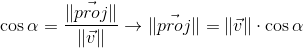
We also already know from the previous paragraph that:
Expressing the cosine of the angle from the second expression, substituting in the first and multiplying by || w || , we get the result: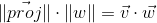
Thus, the scalar product of two vectors is equal to the length of the projection of the vector v on the vector w multiplied by the length of the vector w . A frequent special case of this formula - w has a unit length and, therefore, the scalar product calculates the exact length of the projection.
This interpretation is very important because it shows that the scalar product calculates the coordinates of a point (given by vector v , implying an offset from the origin) along a given axis. The simplest example:
We will use this later when building a transformation into the camera's coordinate system.
Coordinate systems
This section is intended to prepare the basis for the introduction of matrices. I, using the example of the world and local systems, will show for what reasons several coordinate systems are used, rather than one, and how to describe one coordinate system relative to another.
Imagine that we needed to draw a scene with two models, for example:
What coordinate systems naturally follow from such a statement? The first is the coordinate system of the scene itself (which is shown in the figure). This is a coordinate system describing the world that we are going to draw - this is why it is called “world” (in the pictures it will be marked with the word “world”). She "binds" all the objects of the scene together. For example, the coordinates of the center of the object A in this coordinate system are (1, 1) , and the coordinates of the center of the object B are (-1, -1) .
Thus, one coordinate system is already there. Now we need to think about the way in which models come to us, which we will use in the scene.
For simplicity, we assume that the model is described simply as a list of points (“vertices”) of which it consists. For example, model B consists of three points that come to us in the following format:
v 0 = (x 0 , y 0 )
v 1 = (x 1 , y 1 )
v 2 = (x 2 , y 2 )
At first glance, it would be great if they were already described in the “world” system we need! Imagine, you are adding a model to the stage, and it is already where we need it. For model B, it might look like this:
v 0 = (-1.5, -1.5)
v 1 = (-1.0, -0.5)
v 2 = (-0.5, -1.5)
But to use this approach will not work. There is an important reason for this: it makes it impossible to use the same model again in different scenes. Imagine that you were given model B , which was modeled in such a way that when you add it to the stage, it appears in the right place for us, as in the example above. Then, suddenly, the demand has changed - we want to move it to a completely different position. It turns out that the person who created this model will have to move it independently and then give it back to you. Of course, this is complete absurdity. An even stronger argument is that in the case of interactive applications, the model can move, rotate, animate on the stage - what can an artist do a model in all possible positions? That sounds even more stupid.
The solution to this problem is the “local” coordinate system of the model. We model the object in such a way that its center (or that which can be conventionally taken as such) is located at the origin. Then we programmatically orient (move, rotate, etc.) the local coordinate system of the object to the position we need in the world system. Returning to the scene above, object A (unit square, rotated 45 degrees clockwise) can be modeled as follows:
The description of the model in this case will look as follows:
v 0 = (-0.5, 0.5)
v 1 = (0.5, 0.5)
v 2 = (0.5, -0.5)
v 3 = (-0.5, -0.5)
And, accordingly, the position in the scene of two coordinate systems - the world and local object A :
This is one example of why having multiple coordinate systems makes life easier for developers (and artists!). There is another reason - the transition to a different coordinate system can simplify the necessary calculations.
Description of one coordinate system relative to another
There is no such thing as "absolute coordinates". A description of something always happens relative to some kind of coordinate system. Including the description of another coordinate system.
We can build a peculiar hierarchy of coordinate systems in the example above:
 - world space
    - local space (object A)
    - local space (object B)
In our case, this hierarchy is very simple, but in real situations it can have much stronger branching. For example, a local coordinate system of an object may have child systems that are responsible for the position of one or another part of the body.
Each child coordinate system can be described relative to the parent using the following values:
- the origin point of the child system relative to the parent
- coordinates of the basis vectors of the child system relative to the parent
For example, in the picture below, the origin of the system x'y ' (denoted as O' ) is located at (1, 1) , and the coordinates of its base vectors i ' and j' are (0.7, -0.7) and (0.7, 0.7 ) respectively (which roughly corresponds to the axes rotated 45 degrees clockwise).
We do not need to describe the world coordinate system relative to any other, because the world system is the root of the hierarchy, we do not care where it is located or how it is oriented. Therefore, to describe it, we use the standard basis:
Transfer coordinates of points from one system to another
The coordinates of the point P in the parent coordinate system (denoted by P parent ) can be calculated using the coordinates of this point in the child system (denoted as P child ) and the orientation of this child system relative to the parent (described using the origin O and the base vectors i ' and j ' ) as follows:
Let's go back to the example scene above. We orient the local coordinate system of object A relative to the world:
As we already know, in the process of drawing we will need to transfer the coordinates of the vertices of the object from the local coordinate system to the world one. For this we need a description of the local coordinate system relative to the world. It looks like this: the origin is at the point (1, 1) , and the coordinates of the basis vectors are (0.7, -0.7) and (0.7, 0.7) (the method of calculating the coordinates of the basis vectors after the rotation will be described later, so far we have enough result) .
For example, take the first vertex v = (-0.5, 0.5) and calculate its coordinates in the world system:
The fidelity of the result can be seen by looking at the image above.
Matrices
The matrix of dimension mxn is the corresponding dimension table of numbers. If the number of columns in the matrix is equal to the number of rows, then the matrix is called square. For example, a 3 x 3 matrix looks like this:
Matrix Multiplication
Suppose we have two matrices: M (dimension axb ) and N (dimension cxd ). The expression R = M · N is defined only if the number of columns in the matrix M is equal to the number of rows in the matrix N (that is, b = c ). The dimension of the resulting matrix will be equal to axd (i.e., the number of rows is equal to the number of rows M and the number of columns is the number of columns in N ), and the value located at position ij is calculated as the scalar product of the i -th row M by the jth column n :
If the result of multiplying two matrices M · N is defined, then this does not mean that the multiplication in the opposite direction is also determined - N · M (the number of rows and columns may not coincide). In the general case, the operation of matrix multiplication is also not commutative: M · N ≠ N · M.
A unit matrix is a matrix that does not change another matrix multiplied by it (ie, M · I = M ) - a kind of analogue of one for ordinary numbers:
Representation of vectors in the form of matrices
We can also represent a vector as a matrix. There are two possible ways to do this, which are called “row vector” and column vector “”. As the name implies, a row vector is a vector represented as a matrix with one row, and a column vector is a vector represented as a matrix with one column.
Row Vector:
Column Vector:
Further, we will often come across the operation of multiplying the matrix by a vector (which will be explained in the next section), and, running ahead, the matrices with which we will work will have the dimension of either 3 x 3 or 4 x 4 .
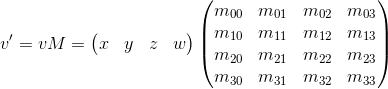
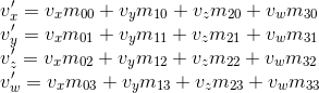
Consider how we can multiply the three-dimensional vector by a 3 x 3 matrix (similar arguments apply for other dimensions). By definition, two matrices can be multiplied if the number of columns in the first matrix equals the number of rows in the second. Thus, since we can represent a vector both as a 1 x 3 matrix (row vector) and as a 3 x 1 matrix (column vector), we get two possible options:
- The multiplication of the vector by the matrix "on the left":
- Multiplying the vector by the matrix "on the right":
As you can see, we get a different result in each case. This can lead to random errors if the API allows you to multiply a vector by a matrix on both sides, because, as we will see later, the transformation matrix implies that the vector will be multiplied by one of two methods. So, in my opinion, the API is better to stick with only one of two options. Within these articles I will use the first option - i.e. the vector is multiplied by the matrix on the left. If you decide to use a different order, then, in order to get correct results, you will need to transpose all the matrices that will later be found in this article, and replace the word “row” with a “column”. It also affects the order of matrix multiplication in the presence of several transformations (it will be discussed in more detail later).
It is also seen from the result of the multiplication that the matrix in a certain way (depending on the value of its elements) changes the vector that was multiplied by it. It can be such transformations as rotation, scaling and others.
Another very important property of the matrix multiplication operation, which will be useful to us later, is distributivity with respect to addition:
Geometric interpretation
As we saw in the previous section, the matrix in a certain way transforms the vector multiplied by it.
Once again, remember that any vector can be represented as a linear combination of basis vectors:
Multiply this expression by the matrix:
Using distributivity with respect to addition, we get:
We have already seen this before, when we considered how to transfer the coordinates of a point from the child system to the parent system, then it looked like this (for three-dimensional space):
There are two differences between these two expressions - in the first expression there is no movement ( O child , we will consider this moment in more detail when we talk about linear and affine transformations), and the vectors i ' , j' and k 'are replaced by iM , jM and kM respectively. Consequently, iM , jM and kM are the basis vectors of the child coordinate system and we transfer the point v child (v x , v y , v y ) from this child coordinate system to the parent ( v transformed = v parent M ).
The transformation process can be depicted as follows using the counterclockwise rotation as an example ( xy is the original, parental coordinate system, x'y ' is a daughter one resulting from the transformation):
Just in case, to make sure that we understand the meaning of each of the vectors used above, we list them again:
- v parent is the vector we initially multiplied by the matrix M. Its coordinates are described relative to the parent coordinate system.
- v child is a vector whose coordinates are equal to the vector v parent , but they are described relative to the child coordinate system. This is the vector v parent transformed in the same way as the basic vectors (since we use the same coordinates)
- v transformed is the same vector as v child but with coordinates recalculated relative to the parent coordinate system. This is the final result of the transformation of the vector v parent
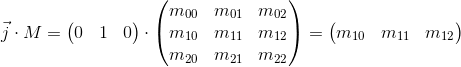
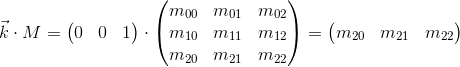
Now consider what happens when you multiply the basis vectors by the matrix M :
It can be seen that the basis vectors of the new child coordinate system obtained as a result of multiplication by the matrix M coincide with the rows of the matrix. This is the very geometric interpretation we were looking for.Now, having seen the transformation matrix, we will know where to look, in order to understand what it is doing - it is enough to present its rows as basis vectors of the new coordinate system. The transformation that occurs with the coordinate system will be the same as the transformation that occurs with the vector multiplied by this matrix.
We can also combine transformations presented in the form of matrices by multiplying them by each other:
Thus, matrices are a very convenient tool for describing and combining transformations.
Linear transformations
To begin, consider the most commonly used linear transformations. Linear transformation is a transformation that satisfies two properties:
An important consequence is that a linear transformation cannot contain displacements (this is also the reason why the O child term was absent in the previous section) because, according to the second formula, 0 is always displayed as 0 .
Rotation
Consider rotation in two-dimensional space. This is a transformation that rotates the coordinate system at a given angle. As we already know, it is enough for us to calculate the new coordinate axes (obtained after rotation at a given angle), and use them as rows of the transformation matrix. The result is easily obtained from the basic geometry:
Example:
The result for rotation in three-dimensional space is obtained in a similar way, with the only difference that we rotate the plane composed of two coordinate axes, and fix the third (around which rotation takes place). For example, the rotation matrix around the x axis looks like this:
Scaling
We can change the scale of the object with respect to all axes using the following matrix: The
axes of the transformed coordinate system will be directed the same way as the original coordinate system, but will require S times the length for one unit of measurement:
Example:
Scaling with the same ratio relative to all axes is called uniform. But we can also scale with different coefficients along different (nonuniform) axes:
Shift
As the name implies, this transformation shifts along the coordinate axis, leaving the remaining axes intact:
Accordingly, the y- axis shift matrix is as follows:
Example:
The matrix for the three-dimensional space is constructed in a similar way. For example, the option for shifting the x axis :
Although this transformation is used very rarely, it will be useful to us in the future when we consider affine transformations.
There is already a decent number of transformations in our stock, which can be represented as a 3 x 3 matrix, but we lack one more — displacement. Unfortunately, it is impossible to express displacement in three-dimensional space using 3 x 3 matrices, since displacement is not a linear transformation. The solution to this problem is homogeneous coordinates, which we will consider later.
Central projection
Our final goal is to draw a three-dimensional scene on a two-dimensional screen. Thus, we need to project our stage onto a plane in one way or another. There are two most commonly used types of projections - orthographic and central (another name is perspective).
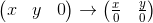
When the human eye looks at the three-dimensional scene, the objects that are farther from it become smaller in the final image, which the person sees - this effect is called perspective. The orthographic projection ignores the perspective, which is a useful feature when working in various CAD systems (as well as in 2D games). The central projection has this property and therefore adds a significant proportion of realism. In this article we will consider only her.
Unlike the orthographic projection, the lines in the perspective projection are not parallel to each other, but intersect at a point called the center of the projection. The center of the projection is the “eye” with which we look at the scene — the virtual camera:
The image is formed on a plane located at a given distance from the virtual camera. Accordingly, the greater the distance from the camera, the larger the projection size:
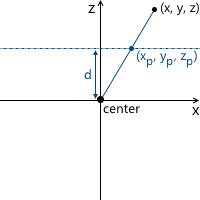
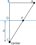
Consider the simplest example: the camera is located at the origin of coordinates, and the projection plane is at a distance d from the camera. We know the coordinates of the point we want to project: (x, y, z) . Find the coordinate x p of the projection of this point on the plane:
This picture shows two similar triangles - CDP and CBA (at three angles):
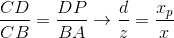
Accordingly, the relationship between the parties remains:
We get the result for the x coordinates:
And, similarly, for the y coordinates:
Later, we will need to use this transformation to form projected image. And here a problem arises - we cannot imagine dividing by z- coordinate in three-dimensional space using a matrix. The solution to this problem, as well as in the case of the displacement matrix, are homogeneous coordinates.
Projective geometry and homogeneous coordinates
To date, we are faced with two problems:
- 3 x 3
Both of these problems solves the use of uniform coordinates. Homogeneous coordinates - a concept from projective geometry. Projective geometry studies projective spaces, and, in order to understand the geometric interpretation of homogeneous coordinates, it is necessary to get to know them.
Below we will consider definitions for two-dimensional projective spaces, since they are easier to portray. Similar reasoning applies to three-dimensional projective spaces (we will use them in the future).
We define a ray in R 3 as follows: a ray is a set of vectors of the form kv ( k is a scalar, v is a non-zero vector, an element of R 3 ). Those.the vector v defines the direction of the ray:
Now we can proceed to the definition of the projective space. The projective plane (i.e., a projective space with a dimension equal to two) P 2 , associated with the space R 3 , is the set of rays in R 3 . Thus, the “point” in P 2 is a ray in R 3 .
Accordingly, two vectors in R 3 set the same element in P 2 , if one of them can be obtained by multiplying the second by a scalar (since in this case they lie on the same ray):
For example, the vectors (1, 1, 1) and (5, 5, 5) represent the same ray, and therefore are the same “point” in the projective plane.
So we came to homogeneous coordinates. Each element in the projective plane is defined by a ray of three coordinates (x, y, w) (the last coordinate is called w instead of z — the generally accepted convention) —the coordinates are called homogeneous and are determined with an accuracy to a scalar. This means that we can multiply (or divide) homogeneous coordinates by a scalar, and they will still represent the same “point” in the projective plane.
In the following, we will use homogeneous coordinates to represent affine (containing displacement) transformations and projections. But before that, one more question needs to be solved: how to represent in the form of homogeneous coordinates the vertices of the model already given to us? Since the “addition” to the homogeneous coordinates occurs due to the addition of the third coordinate w , the question boils down to what value of w we need to use. The answer to this question is any non-zero. The difference in the use of different values of w is the convenience of working with them.
And, as will be understood later (and partly clear intuitively), the most convenient value of w is one. The advantages of this choice are as follows:
- ( )
- ( ) w , (.. w):
— w = 1 , w — , w
Thus, we choose the value w = 1 , which means that our input data in homogeneous coordinates will now look like this (of course, we’ve already added one, and will not be in the model description itself):
v 0 = (x 0 , y 0 , 1)
v 1 = (x 1 , y 1 , 1)
v 2 = (x 2 , y 2 , 1)
Now we need to consider a special case when working with the w- coordinate. Namely - its equality to zero. Above we said that we can choose any value of w, not equal to zero, for expansion to homogeneous coordinates. We cannot take w = 0 , in particular, because it will not allow moving this point (since, as we will see later, the movement occurs precisely due to the value in the w coordinate). Also, if the w coordinate of the point is zero, we can consider it as a point "at infinity", because when we try to return to the plane w = 1, we get the division by zero:
And, although we cannot use the zero value for the model vertices, we can use it for vectors! This will lead to the fact that the vector will not be subject to movement during transformations - which makes sense, because the vector does not describe the position. For example, when transforming the normal, we cannot move it, otherwise we will get an incorrect result. We will take a closer look at this when the need arises to transform vectors.
In this connection, it is often written that for w = 1 we describe a point, and for w = 0 , a vector.
As I already wrote, we used the example of two-dimensional projective projective spaces, but in fact we will use three-dimensional projective spaces, which means each point will be described by 4 coordinates: (x, y, z, w) .
Moving using homogeneous coordinates
Now we have all the necessary tools to describe affine transformations. Affine transformations are linear transformations with subsequent displacement. They can be described as follows:
We can also use 4 x 4 matrices to describe affine transformations using homogeneous coordinates:
Consider the result of multiplying the vector, represented as homogeneous coordinates, and multiplying by 4 x 4 matrix:
As you can see, the difference from the transformation , represented in the form of a 3 x 3 matrix, consists in the presence of the 4th coordinate, as well as the new terms in each of the coordinates of the form v w · m 3i . Using this, and implying w = 1, we can imagine the movement as follows:
Here you can make sure that the choice of w = 1 is correct . To represent the displacement dx, we use a term of the form w · dx / w . Accordingly, the last row of the matrix looks like (dx / w, dy / w, dz / w, 1) . In the case of w = 1, we can simply omit the denominator.
This matrix also has a geometric interpretation. Recall the shift matrix, which we considered earlier. It has exactly the same format, the only difference is that the fourth axis is shifted, thus shifting the three-dimensional subspace located in the hyperplane w = 1 by the corresponding values.
Description of the virtual camera
A virtual camera is the “eye” with which we look at the scene. Before proceeding further, it is necessary to understand how to describe the position of the camera in space, and what parameters are necessary for the formation of the final image.
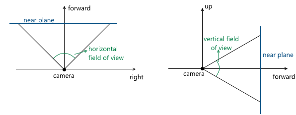
The camera parameters set the truncated view pyramid (view frustum), which determines which part of the scene falls into the final image:
Consider them in turn:
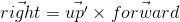
- . , , . . «UVN» , .. . , u , v n ( ), right , up forward — , . .
API — . , , up ( up' ). :- right forward up' :
- up , right forward :

, up' forward , up . OpenGL, gluLookAt .
— , - right forward up' :
- z - (near/far clipping plane)
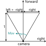
- Camera viewing angles. They set the dimensions of the truncated view pyramid:
Since the scene will later be projected onto the projection plane, the image on this plane will later be displayed on the computer screen. Therefore, it is important that the aspect ratio of this plane and the window (or part thereof) in which the image will be shown coincides. This can be achieved by giving the API user the ability to set only one viewing angle, and the second to calculate in accordance with the aspect ratio of the window. For example, knowing the horizontal viewing angle, we can calculate the vertical as follows: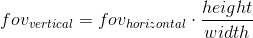
When we discussed the central projection, we saw that the farther the projection plane from the camera, the larger the size of the resulting image - we denoted the distance from the camera (assuming that it is located at the origin) along the z axis from the projection plane of the variable d . Accordingly, the question should be solved, what value of d we need to choose. In fact, any non-zero. Despite the fact that the image size increases with increasing d , that part of the projection plane, which intersects with the pyramid of view, increases proportionally, leaving the same image scale relative to the dimensions of this part of the plane. In the future, we will use d = 1 for convenience.
Example in 2D:
As a result, for zooming, we need to change the viewing angles - this will change the size of the part of the projection plane that intersects with the pyramid of the review, leaving the projection size the same.
We can move and rotate the camera, changing the position and orientation of its coordinate system. Code example:
Hidden text
void camera::move_right(float distance) { m_position += m_right * distance; } void camera::move_left(float const distance) { move_right(-distance); } void camera::move_up(float const distance) { m_position += m_up * distance; } void camera::move_down(float const distance) { move_up(-distance); } void camera::move_forward(float const distance) { m_position += m_forward * distance; } void camera::move_backward(float const distance) { move_forward(-distance); } void camera::yaw(float const radians) { matrix3x3 const rotation{matrix3x3::rotation_around_y_axis(radians)}; m_forward = m_forward * rotation; m_right = m_right * rotation; m_up = m_up * rotation; } void camera::pitch(float const radians) { matrix3x3 const rotation{matrix3x3::rotation_around_x_axis(radians)}; m_forward = m_forward * rotation; m_right = m_right * rotation; m_up = m_up * rotation; } Graphics pipeline
Now we have all the necessary foundation in order to describe by steps the steps that are necessary to obtain an image of a three-dimensional scene on a computer screen. For simplicity, we will assume that the pipeline draws one object at a time.
Incoming parameters of the pipeline:
- Object and its orientation in the world coordinate system
- The camera whose parameters we will use when composing the image
1. Transition to the world coordinate system
At this stage, we transform the object vertices from the local coordinate system into the world one.
Suppose that the orientation of an object in the world coordinate system is defined by the following parameters:
- At what point in the world coordinate system is the object: (x world , y world , z world )
- How the object is rotated: (r x , r y , r z )
- Object scale: (s x , s y , s z )
We call the matrices of these transformations T , R, and S, respectively. To obtain the final matrix, which will transform an object into a world coordinate system, we need only to multiply them. It is important to note here that the order of multiplication of matrices plays a role - this directly follows from the fact that the multiplication of matrices is noncommutative.
Recall that scaling occurs relative to the origin. If we first displace the object to the desired point, and then apply a scale to it, we will get the wrong result - the position of the object will change again after scaling. A simple example:
A similar rule applies with respect to rotation - it occurs relative to the origin, which means that the position of the object will change if we first make a movement.
Thus, the correct sequence in our case is as follows: scaling - rotation - offset:
2. Transition to camera coordinate system
The transition to the camera's coordinate system, in particular, is used to simplify further calculations. In this coordinate system, the camera is located at the origin, and its axes are the forward , right , up vectors, which we considered in the previous section.
The transition to the camera coordinate system consists of two steps:
- Move the world so that the position of the camera coincides with the origin
- Using the calculated axes right , up , forward , we calculate the coordinates of the object's vertices along these axes (this step can be viewed as a rotation of the camera's coordinate system so that it coincides with the world coordinate system)
The first step can be easily represented as a matrix of displacement on (-pos x , -pos y , -pos z ) , where pos is the position of the camera in the world coordinate system:
To implement the second item, we use the property of the scalar product, which we considered at the very beginning - the scalar product calculates the length of the projection along a given axis. Thus, in order to transfer point A to the camera's coordinate system (taking into account the fact that the camera is at the origin, we did this in the first paragraph), we just need to take its scalar product with the vectors right , up , forward . Denote a point in the world coordinate system v , and the same point translated into the camera coordinate system, v ' , then:
This operation can be represented as a matrix:
Combining these two transformations, we get the transition matrix to the camera coordinate system:
Schematically, this process can be depicted as follows:
3. Transition to homogeneous clipping space and normalization of coordinates
As a result of the previous point, we obtained the coordinates of the object's vertices in the camera's coordinate system. The next thing to do is to make a projection of these vertices on the plane and “cut off” the extra vertices. The vertex of the object is cut off if it lies outside the pyramid of the review (i.e. its projection does not lie on that part of the plane which the pyramid of the survey covers). For example, vertex v 1 in the figure below:
Both of these tasks are partially solved by the projection matrix. “Partially” - because it does not produce the projection itself, but prepares the w- coordinate of the vertex for this. Because of this, the name “projection matrix” does not sound very appropriate (although this is a fairly common term), and I will call it the clip matrix in the future, since it also displays the truncated view pyramid in a uniform clipping space (homogeneous clip space).
But first things first. So, the first is preparation for the projection. For this, we put the z- coordinate of the vertex in its w- coordinate. The projection itself (that is, division by z ) will occur upon further normalization of the w-coordinate — that is, when returning to the space w = 1 .
The next thing this matrix has to do is translate the coordinates of the vertices of the object from the camera space into a homogeneous clip space. This space, the coordinates of the non-clipped vertices in which are such that after applying the projection (i.e., dividing by the w- coordinate, since we saved the old z- coordinate in it), the coordinates of the vertex are normalized; satisfy the following conditions:
Inequality for z coordinates can vary for different APIs. For example, in OpenGL, it corresponds to what is above. In Direct3D, the z coordinate is displayed in the interval [0, 1] . We will use the OpenGL interval, i.e. [-1, 1] .
Such coordinates are called normalized device coordinates (normalized device coordinates or simply NDC).
Since we obtain the NDC coordinates by dividing the coordinates by w , the vertices in the cut-off space satisfy the following conditions:
Thus, by transferring the vertices to this space, we can find out whether it is necessary to cut the vertex simply by checking its coordinates for the inequalities above. Any vertex that does not satisfy these conditions must be cut off. The cut-off itself is a topic for a separate article, because its correct implementation leads to the creation of new vertices. So far, as a quick fix, we will not draw a face if at least one of its vertices is clipped. Of course, the result will not be very neat. For example, for a car model, it looks like this:
Total, this stage consists of the following steps:
- Get vertices in camera space
- Multiply by the clipping matrix - go to the clipping space
- Mark clipped vertices by checking for the inequalities described above.
- We divide the coordinates of each vertex into its w- coordinate - go to the normalized coordinates
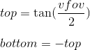
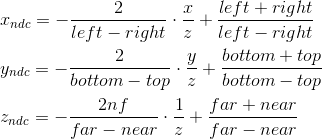
Now consider how we map the coordinates from the camera space to the clipping space. Recall that we decided to use the projection plane z = 1 . First we need to find a function that displays the coordinates lying on the intersection of the pyramid of the review and the projection plane in the interval [-1, 1] . For this we find the coordinates of the points defining this part of the plane. These two points have coordinates (left, top) and (right, bottom) . We will consider only the case when the pyramid of view is symmetrical about the direction of the camera.
We can calculate them using viewing angles:
We get:
Similarly for top and bottom :
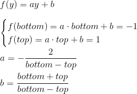
Thus, we need to display the interval [left, right] , [bottom, top] , [near, far] in [-1; 1] . Find a linear function that gives this result for left and right :
Similarly, the function for the bottom and top is obtained:
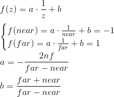
The expression for z is different. Instead of considering a function of the form az + b, we will consider the function a · 1 / z + b , because later, when we implement the depth buffer, we will need to linearly interpolate the inverse of the z-coordinate. We will not consider this issue now, and just take it for this. We get:
Thus, we can write that the normalized coordinates are obtained as follows from the coordinates in the camera space:
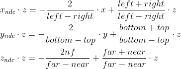
We cannot immediately apply these formulas, because division by z will occur later, with normalization of w- coordinates. We can use this, and instead calculate the following values (multiplying by z), which after dividing by w , will result in normalized coordinates:
It is by these formulas that we transform into the cut-off space. We can write this transformation in matrix form (remembering additionally that we put z in the w coordinate):
Transition to screen coordinate system
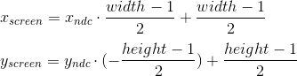
To the current stage, we have the coordinates of the object vertices in the NDC. We need to translate them into screen coordinate system. Recall that the upper left corner of the projection plane was mapped to (-1, 1), and the lower right to (1, -1). For the screen, I will use the upper left corner as the origin of the coordinate system, with the axes pointing right and down:
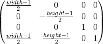
This viewport transformation can be made using simple formulas:
Or, in matrix form:
We will leave using z ndc until the implementation of the depth buffer.
As a result, we have the coordinates of the vertices on the screen, which we use for drawing.
Implementation in code
Below is an example of code that implements a pipeline using the method described above and performing drawing in wireframe mode (i.e., simply connecting vertices with lines). It also implies that the object is described by a set of vertices and a set of indexes of the vertices (faces) of which its polygons consist:
Hidden text
void pipeline::draw_mesh( std::shared_ptr<mesh const> mesh, vector3 const& position, vector3 const& rotation, camera const& camera, bitmap_painter& painter) const { matrix4x4 const local_to_world_transform{ matrix4x4::rotation_around_x_axis(rotation.x) * matrix4x4::rotation_around_y_axis(rotation.y) * matrix4x4::rotation_around_z_axis(rotation.z) * matrix4x4::translation(position.x, position.y, position.z)}; matrix4x4 const camera_rotation{ camera.get_right().x, camera.get_up().x, camera.get_forward().x, 0.0f, camera.get_right().y, camera.get_up().y, camera.get_forward().y, 0.0f, camera.get_right().z, camera.get_up().z, camera.get_forward().z, 0.0f, 0.0f, 0.0f, 0.0f, 1.0f}; matrix4x4 const camera_translation{ 1.0f, 0.0f, 0.0f, 0.0f, 0.0f, 1.0f, 0.0f, 0.0f, 0.0f, 0.0f, 1.0f, 0.0f, -camera.get_position().x, -camera.get_position().y, -camera.get_position().z, 1.0f}; matrix4x4 const world_to_camera_transform{camera_translation * camera_rotation}; float const projection_plane_z{1.0f}; float const near{camera.get_near_plane_z()}; float const far{camera.get_far_plane_z()}; float const right{std::tan(camera.get_horizontal_fov() / 2.0f) * projection_plane_z}; float const left{-right}; float const top{std::tan(camera.get_vertical_fov() / 2.0f) * projection_plane_z}; float const bottom{-top}; matrix4x4 const camera_to_clip_transform{ 2.0f * projection_plane_z / (right - left), 0.0f, 0.0f, 0.0f, 0.0f, 2.0f * projection_plane_z / (top - bottom), 0.0f, 0.0f, (left + right) / (left - right), (bottom + top) / (bottom - top), (far + near) / (far - near), 1.0f, 0.0f, 0.0f, -2.0f * near * far / (far - near), 0.0f}; matrix4x4 const local_to_clip_transform{ local_to_world_transform * world_to_camera_transform * camera_to_clip_transform}; std::vector<vector4> transformed_vertices; for (vector3 const& v : mesh->get_vertices()) { vector4 v_transformed{vector4{vx, vy, vz, 1.0f} * local_to_clip_transform}; if ((v_transformed.x > v_transformed.w) || (v_transformed.x < -v_transformed.w)) { mark_vector4_as_clipped(v_transformed); } else if ((v_transformed.y > v_transformed.w) || (v_transformed.y < -v_transformed.w)) { mark_vector4_as_clipped(v_transformed); } else if ((v_transformed.z > v_transformed.w) || (v_transformed.z < -v_transformed.w)) { mark_vector4_as_clipped(v_transformed); } transformed_vertices.push_back(v_transformed); } float const width{static_cast<float>(painter.get_bitmap_width())}; float const height{static_cast<float>(painter.get_bitmap_height())}; matrix4x4 const ndc_to_screen{ width / 2.0f, 0.0f, 0.0f, 0.0f, 0.0f, -height / 2.0f, 0.0f, 0.0f, 0.0f, 0.0f, 1.0f, 0.0f, width / 2.0f, height / 2.0f, 0.0f, 1.0f}; for (vector4& v : transformed_vertices) { if (is_vector4_marked_as_clipped(v)) { continue; } float const w_reciprocal{1.0f / vw}; vx *= w_reciprocal; vy *= w_reciprocal; vz *= w_reciprocal; vw = 1.0f; v = v * ndc_to_screen; } for (face const& f : mesh->get_faces()) { vector4 const& v1{transformed_vertices[f.index1]}; vector4 const& v2{transformed_vertices[f.index2]}; vector4 const& v3{transformed_vertices[f.index3]}; bool const v1_clipped{is_vector4_marked_as_clipped(v1)}; bool const v2_clipped{is_vector4_marked_as_clipped(v2)}; bool const v3_clipped{is_vector4_marked_as_clipped(v3)}; if (!v1_clipped && !v2_clipped) { painter.draw_line( point2d{static_cast<unsigned int>(v1.x), static_cast<unsigned int>(v1.y)}, point2d{static_cast<unsigned int>(v2.x), static_cast<unsigned int>(v2.y)}, color{255, 255, 255}); } if (!v3_clipped && !v2_clipped) { painter.draw_line( point2d{static_cast<unsigned int>(v2.x), static_cast<unsigned int>(v2.y)}, point2d{static_cast<unsigned int>(v3.x), static_cast<unsigned int>(v3.y)}, color{255, 255, 255}); } if (!v1_clipped && !v3_clipped) { painter.draw_line( point2d{static_cast<unsigned int>(v3.x), static_cast<unsigned int>(v3.y)}, point2d{static_cast<unsigned int>(v1.x), static_cast<unsigned int>(v1.y)}, color{255, 255, 255}); } } } An example of using SDL2 for implementation
In this section, I will briefly explain how SDL2 can be used to implement rendering.
Texture initialization
The first is, of course, the initialization of the library and the creation of the window. If only graphics are needed from SDL, then you can initialize with the SDL_INIT_VIDEO flag:
Hidden text
if (SDL_Init(SDL_INIT_VIDEO) < 0) { throw std::runtime_error(SDL_GetError()); } m_window = SDL_CreateWindow( "lantern", SDL_WINDOWPOS_UNDEFINED, SDL_WINDOWPOS_UNDEFINED, width, height, SDL_WINDOW_SHOWN); if (m_window == nullptr) { throw std::runtime_error(SDL_GetError()); } m_renderer = SDL_CreateRenderer(m_window, -1, SDL_RENDERER_ACCELERATED); if (m_renderer == nullptr) { throw std::runtime_error(SDL_GetError()); } Then, create a texture into which we will render. I will use the ARGB8888 format, which means that each pixel in the texture will be allocated 4 bytes - three bytes on the RGB channels, and one on the alpha channel.
Hidden text
m_target_texture = SDL_CreateTexture( m_renderer, SDL_PIXELFORMAT_ARGB8888, SDL_TEXTUREACCESS_STREAMING, width, height); if (m_target_texture == nullptr) { throw std::runtime_error(SDL_GetError()); } You need to remember to “clear” the SDL and all variables taken from it when the application exits:
Hidden text
if (m_target_texture != nullptr) { SDL_DestroyTexture(m_target_texture); m_target_texture = nullptr; } if (m_renderer != nullptr) { SDL_DestroyRenderer(m_renderer); m_renderer = nullptr; } if (m_window != nullptr) { SDL_DestroyWindow(m_window); m_window = nullptr; } SDL_Quit(); Drawing, display on the screen
We can use SDL_UpdateTexture to update the texture, which we will then display on the screen. This function accepts, among others, the following parameters:
- Data is an array of bytes, which is an array of pixels with corresponding values.
- The number of bytes in one line of the image (pitch) is calculated as the number of pixels multiplied by 4 (because the format is ARGB8888 )
It is logical to allocate the drawing functionality to the texture, represented by an array of bytes, in a separate class. It will allocate memory for the array, clear the texture, draw pixels and lines. Drawing a pixel can be done as follows (the order of bytes differs depending on SDL_BYTEORDER ):
Hidden text
void bitmap_painter::draw_pixel(point2d const& point, color const& c) { unsigned int const pixel_first_byte_index{m_pitch * point.y + point.x * 4}; #if SDL_BYTEORDER == SDL_BIG_ENDIAN m_data[pixel_first_byte_index + 0] = cb; m_data[pixel_first_byte_index + 1] = cg; m_data[pixel_first_byte_index + 2] = cr; // m_data[pixel_first_byte_index + 3] is alpha, we don't use it for now #else // m_data[pixel_first_byte_index + 0] is alpha, we don't use it for now m_data[pixel_first_byte_index + 1] = cr; m_data[pixel_first_byte_index + 2] = cg; m_data[pixel_first_byte_index + 3] = cb; #endif } Line drawing can be implemented, for example, by the Brezenham algorithm .
After using SDL_UpdateTexture , you must copy the texture into SDL_Renderer and display it on the screen using SDL_RenderPresent . Together:
Hidden text
SDL_UpdateTexture(m_target_texture, nullptr, m_painter.get_data(), m_painter.get_pitch()); SDL_RenderCopy(m_renderer, m_target_texture, nullptr, nullptr); SDL_RenderPresent(m_renderer); That's all. Link to the project: https://github.com/loreglean/lantern .
Source: https://habr.com/ru/post/243011/
All Articles