How recommender systems work. Lecture in Yandex
Hi, my name is Michael Roizner. Recently, I gave a lecture to students of Small Shad Yandex about what recommendation systems are and what methods are there. Based on the lecture, I prepared this post.
Lecture plan:
Let's start with a simple one: what are recommender systems in general, and how they are. Probably everyone has already come across them on the Internet. The first example is movie recommendation systems.
')

On imdb.com, users can rate movies on a ten-point scale. Ratings are aggregated, it turns out the average movie rating. On the same site there is a block with recommendations for a specific user. If I went to the site and rated several films, imdb will be able to recommend me some more films. A similar block is on Facebook.
Something similar, but only for music, does last.fm. He recommends me artists, albums, events that I should go to. The Pandora service in Russia is almost unknown, since it does not work with us, but in America it is very popular. This is a personal radio, which gradually adapts to the user based on his ratings, and as a result plays only those tracks that he likes.

Another well-known area is product recommendation. In the picture below we have, of course, Amazon. If you bought something on Amazon, you will be hunted with additional offers: similar products or accessories. This is also good for users (they don’t need to search for these products on their own), and of course, this is good for the store itself.

We have listed three categories, but in fact they are much more: places on the map, news, articles, websites, concerts, theaters, exhibitions, videos, books, apps, games, travel, social connections and much more.
There are two main types of recommender systems. Of course, there are more of them, but today we will consider these and especially the collaborative filtering.
Recommender systems appeared on the Internet for a long time, about 20 years ago. However, the real upswing in this area happened about 5-10 years ago when the Netflix Prize competition took place. Netflix did not rent digital copies at that time, but sent out VHS tapes and DVDs. For them it was very important to improve the quality of the recommendations. The better Netflix recommends movies to its users, the more films they rent. Accordingly, the company's profit grows. In 2006, they launched the Netflix Prize competition. They posted openly the collected data: about 100 million marks on a five-point scale, indicating the ID of the users who put them. The participants of the competition should have foreseen as best as possible what assessment a particular user would give to a certain film. The quality of the prediction was measured using the RMSE (mean square deviation) metric. Netflix already had an algorithm that predicted user ratings with a quality of 0.9514 using the RMSE metric. The task was to improve the prediction by at least 10% - to 0.8563. The winner was promised a prize of $ 1,000,000. The competition lasted about three years. For the first year, the quality was improved by 7%, then everything slowed down a bit. But at the end, two teams sent their solutions with a difference of 20 minutes, each of which passed a threshold of 10%, the quality was the same with the accuracy of the fourth mark. In the task, over which many teams had been beating for three years, everyone decided some twenty minutes. The late team (like many others who participated in the competition) was left with nothing, but the competition itself very strongly spurred development in this area.
To begin, we formalize our problem. What we have? We have a set of users 𝑢 ∈ 𝑈, a set of objects 𝑖 ∈ 𝐼 (movies, tracks, products, etc.) and a set of events (𝑟 𝑢𝑖 , 𝑢, 𝑖, ...) ∈ 𝒟 (actions that users perform with objects). Each event is set by user 𝑢, object 𝑖, its result 𝑟 𝑢𝑖 and, possibly, some other characteristics. We are required to:
Suppose we are given a table with user ratings:

You need to predict as best you can what ratings should be in the cells with question marks:
Recall that the main idea of collaborative filtering is that similar users usually like similar objects. Let's start with the simplest method.

This algorithm has several problems:
Let's try to slightly improve the previous method and replace hard clustering with the following formula:
However, this algorithm also has its own problems:
There is an absolutely symmetric algorithm:
In the previous method, we were repelled by the idea that, say, the user would like the movie if his friends liked it. Here we believe that the user will like the movie if he liked similar movies.
Problems:
All of these methods have the following disadvantages:
Therefore, we turn to a more complex algorithm, which is almost devoid of these shortcomings.
For this algorithm, we need several concepts from linear algebra: vectors, matrices, and operations with them. I will not give here all the definitions, if you need to refresh this knowledge, then all explanations are in the video of the lecture from about 33 minutes.
SVD (Singular Value Decomposition), translated as a singular decomposition of the matrix. The singular decomposition theorem states that any matrix 𝐀 of size 𝑛 × 𝑚 has a decomposition into a product of three matrices: 𝑈, Ʃ and 𝑉 𝑇 :

The matrices 𝑈 and 𝑉 are orthogonal, and Ʃ is diagonal (although not square).
Moreover, the lambda in the matrix Ʃ will be ordered by non-increasing. Now we will not prove this theorem, just use the decomposition itself.
But what do we have from the fact that we can some kind of matrix in the product of three even more incomprehensible matrices. For us, the following will be interesting. In addition to the usual decomposition, it is still truncated, when among the lambdas, only the first 𝑑 numbers remain, and the rest we assume to be zero.

This is equivalent to the fact that for matrices 𝑈 and 𝑉 we leave only the first
columns, and the matrix Ʃ is cut to square 𝑑 × 𝑑.
So, it turns out that the obtained matrix 𝐀 ′ well approximates the original matrix 𝐀 and, moreover, is the best low-rank approximation in terms of the standard deviation.
How to use all this for recommendations? We had a matrix, we decomposed it into a product of three matrices. What is not exactly laid out, and approximately. Simplify everything a bit by designating the product of the first two matrices for a single matrix:

Now let's digress a little from all these matrices and concentrate on the resulting algorithm: to predict the user's rating 𝑈 for the movie , we take some vector 𝑝 𝑢 (set of parameters) for this user and vector for this movie 𝑖 . Their scalar product will be the prediction we need: 𝑟̂ 𝑢𝑖 = ⟨𝑝 𝑢 , 𝑞 𝑖⟩ .
The algorithm is quite simple, but it gives surprising results. It does not just allow us to predict estimates. Using it, we can identify hidden signs of objects and user interests by user history. For example, it may happen that at the first coordinate of the vector each user will have a number indicating whether the user looks more like a boy or a girl, the second coordinate is a number reflecting the approximate age of the user. At the same film, the first coordinate will show whether it is more interesting to boys or girls, and the second one - to what age group of users it is interesting.
But not everything is so simple. There are a few problems. First, the estimation matrix is not completely known to us, so we cannot simply take its SVD decomposition. Secondly, the SVD decomposition is not unique: (𝑈Ω) Ʃ (𝑉Ω) = 𝑈Ʃ𝑉 𝑇 , so even if we find at least some decomposition, it is unlikely that the first coordinate in it will correspond to the gender of the user, and the second will be the age.
Let's try to deal with the first problem. Here we need machine learning. So, we cannot find the SVD decomposition of the matrix, since we do not know the matrix itself. But we want to take advantage of this idea and come up with a prediction model that will work in a manner similar to SVD. Our model will depend on many parameters - vectors of users and movies. For the given parameters, in order to predict the estimate, we take the user vector, the vector of the film and get their scalar product:

But since we do not know vectors, they still need to be obtained. The idea is that we have user ratings with which we can find the optimal parameters for which our model would predict these ratings as best we can:

So, we want to find such parameters θ so that the error square is as small as possible. But there is a paradox here: we want to make less mistakes in the future , but we do not know what estimates we will ask. Accordingly, we cannot optimize this. But we already know the ratings given by users. Let's try to choose the parameters so that on those estimates that we already have, the error was as small as possible. In addition, we add another term - the regularizer.

Regularization is needed to combat retraining - a phenomenon when the constructed model well explains the examples from the training set, but it does not work well with examples that did not participate in the training. In general, there are several methods to combat retraining; I would like to mention two of them. First, you need to choose simple models. The simpler the model, the better it summarizes the future data (this is similar to the well-known principle of Occam's razor). And the second method is just regularization. When we set up a model for a training set, we optimize the error. Regularization is that we optimize not just an error, but an error plus some function of the parameters (for example, the norm of the vector of parameters). This allows you to limit the size of the parameters in the solution, reduces the degree of freedom of the model.
How do we find the optimal parameters? We need to optimize this functionality:
There are many parameters: for each user, for each object we have our own vector, which we want to optimize. We have a function depending on a large number of variables. How to find her minimum? Here we need a gradient - a vector of partial derivatives for each parameter.
Gradient is very convenient to visualize. The illustration shows the surface: a function of two variables. For example, the altitude above sea level. Then the gradient at any particular point is a vector directed in the direction where our function grows the most. And if you run water from this point, it will flow in the direction opposite to the gradient.

The most well-known method for optimizing functions is gradient descent. Suppose we have a function of many variables, we want to optimize it. We take some initial value, and then we look where we can move in order to minimize this value. The gradient descent method is an iterative algorithm: it repeatedly takes the parameters of a certain point, looks at the gradient and steps against its direction:

The problems with this method lie in the fact that, firstly, in our case, it works very slowly and, secondly, it finds local, rather than global, minima. The second problem is not so terrible for us, because In our case, the value of the functional in local minima is close to the global optimum.
However, the gradient descent method is not always necessary. For example, if we need to calculate the minimum for a parabola, there is no need to act by this method, we know for sure where its minimum is. It turns out that the functionality that we are trying to optimize - the sum of the squares of errors plus the sum of the squares of all parameters - is also a quadratic functional, it is very similar to a parabola. For each specific parameter, if we fix all the others, it will be just a parabola. Those. at least one coordinate we can accurately determine. The Alternating Least Squares method is based on this consideration. I will not dwell on it in detail. Let me just say that in it we alternately accurately find minima in one coordinate or another:

We fix all the parameters of the objects, optimize exactly the parameters of the users, further fix the parameters of the users and optimize the parameters of the objects. We act iteratively:

It all works quickly enough, with each step can be parallelized.
If we want to improve the quality of recommendations, we need to learn how to measure it. For this, an algorithm trained on one sample — a training one — is tested on another - a test one. Netflix suggested measuring the quality of recommendations for the RMSE metric:

Today it is the standard metric for predicting an estimate. However, it has its drawbacks:
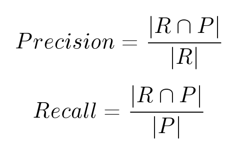
There are other metrics - ranking metrics, for example, based on completeness and accuracy. Let 𝑹 be the set of recommended objects, 𝑷 the set of objects that the user will actually like.
There are also problems here:
It turns out that the perception of recommendations is influenced not only by the quality of ranking, but also by some other characteristics. Among them, for example, variety (you should not give the user movies only on one topic or from one series), surprise (if you recommend very popular movies, such recommendations will be too banal and almost useless), novelty (many people like classic films, but recommendations usually used to discover something new) and many others.
Similarity of objects is not such an obvious thing. There are different approaches to this task:
Lecture plan:
- Types and applications of recommender systems.
- The simplest algorithms.
- Introduction to linear algebra.
- Svd algorithm.
- Measuring the quality of recommendations.
- Development direction.
Let's start with a simple one: what are recommender systems in general, and how they are. Probably everyone has already come across them on the Internet. The first example is movie recommendation systems.
')
On imdb.com, users can rate movies on a ten-point scale. Ratings are aggregated, it turns out the average movie rating. On the same site there is a block with recommendations for a specific user. If I went to the site and rated several films, imdb will be able to recommend me some more films. A similar block is on Facebook.
Something similar, but only for music, does last.fm. He recommends me artists, albums, events that I should go to. The Pandora service in Russia is almost unknown, since it does not work with us, but in America it is very popular. This is a personal radio, which gradually adapts to the user based on his ratings, and as a result plays only those tracks that he likes.
Another well-known area is product recommendation. In the picture below we have, of course, Amazon. If you bought something on Amazon, you will be hunted with additional offers: similar products or accessories. This is also good for users (they don’t need to search for these products on their own), and of course, this is good for the store itself.
We have listed three categories, but in fact they are much more: places on the map, news, articles, websites, concerts, theaters, exhibitions, videos, books, apps, games, travel, social connections and much more.
Types of recommendation systems
There are two main types of recommender systems. Of course, there are more of them, but today we will consider these and especially the collaborative filtering.
- Content-based
- The user is recommended objects similar to those that this user has already used.
- Similarities are evaluated by feature content.
- Strong dependence on the subject area, the usefulness of the recommendations is limited.
- Collaborative Filtering
- The recommendation is based on the history of assessments of both the user and other users.
- A more universal approach often gives better results.
- There are problems (for example, cold start).
Recommender systems appeared on the Internet for a long time, about 20 years ago. However, the real upswing in this area happened about 5-10 years ago when the Netflix Prize competition took place. Netflix did not rent digital copies at that time, but sent out VHS tapes and DVDs. For them it was very important to improve the quality of the recommendations. The better Netflix recommends movies to its users, the more films they rent. Accordingly, the company's profit grows. In 2006, they launched the Netflix Prize competition. They posted openly the collected data: about 100 million marks on a five-point scale, indicating the ID of the users who put them. The participants of the competition should have foreseen as best as possible what assessment a particular user would give to a certain film. The quality of the prediction was measured using the RMSE (mean square deviation) metric. Netflix already had an algorithm that predicted user ratings with a quality of 0.9514 using the RMSE metric. The task was to improve the prediction by at least 10% - to 0.8563. The winner was promised a prize of $ 1,000,000. The competition lasted about three years. For the first year, the quality was improved by 7%, then everything slowed down a bit. But at the end, two teams sent their solutions with a difference of 20 minutes, each of which passed a threshold of 10%, the quality was the same with the accuracy of the fourth mark. In the task, over which many teams had been beating for three years, everyone decided some twenty minutes. The late team (like many others who participated in the competition) was left with nothing, but the competition itself very strongly spurred development in this area.
Simple algorithms
To begin, we formalize our problem. What we have? We have a set of users 𝑢 ∈ 𝑈, a set of objects 𝑖 ∈ 𝐼 (movies, tracks, products, etc.) and a set of events (𝑟 𝑢𝑖 , 𝑢, 𝑖, ...) ∈ 𝒟 (actions that users perform with objects). Each event is set by user 𝑢, object 𝑖, its result 𝑟 𝑢𝑖 and, possibly, some other characteristics. We are required to:
- predict preference:
𝑟̂ 𝑢𝑖 = Predict (𝑢, 𝑖, ...) ≈ 𝑟 𝑢𝑖 . - personal recommendations:
𝑢 ⟼ (𝑖 1 , ..., 𝑖 𝘒 ) = Recommend (, ...). - similar objects:
⟼ (𝑖 1 , ..., 𝑖 𝑀 ) = Similar 𝑀 ().
Rating table
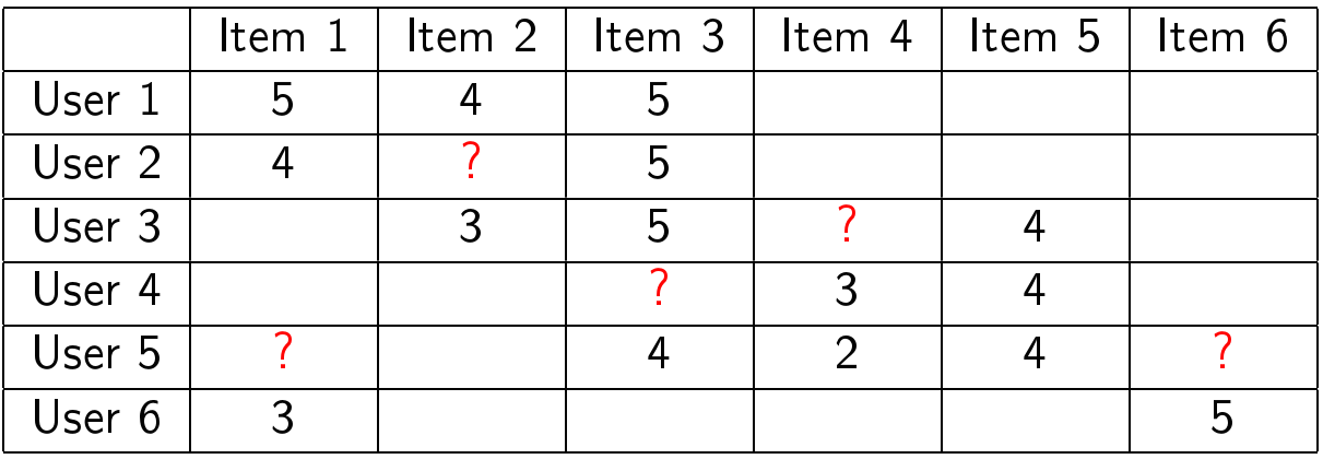
Suppose we are given a table with user ratings:
You need to predict as best you can what ratings should be in the cells with question marks:
User clustering
Recall that the main idea of collaborative filtering is that similar users usually like similar objects. Let's start with the simplest method.
- Choose a conditional measure of similarity of users according to their rating history 𝑠𝑖𝑚 (𝑢, 𝑣).
- We will unite users into groups (clusters) so that similar users will end up in the same cluster: 𝑢 ⟼ 𝐹 (𝑢).
- The user’s score for an object will be predicted as the average cluster rating for this object:
This algorithm has several problems:
- Nothing to recommend to new / atypical users. For such users, there is no suitable cluster with similar users.
- It does not take into account the specificity of each user. In a sense, we divide all users into some classes (templates).
- If nobody in the cluster has evaluated the object, then the prediction will fail.
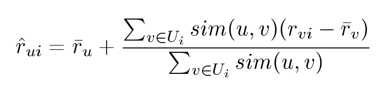
User-based
Let's try to slightly improve the previous method and replace hard clustering with the following formula:
However, this algorithm also has its own problems:
- Nothing to recommend to new / atypical users. For these users, we still can not find similar.
- Cold start - new objects are not recommended to anyone.
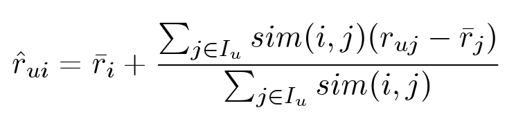
Item-based
There is an absolutely symmetric algorithm:
In the previous method, we were repelled by the idea that, say, the user would like the movie if his friends liked it. Here we believe that the user will like the movie if he liked similar movies.
Problems:
- Cold start - new objects are not recommended to anyone.
- Recommendations are often trivial.
Common problems of the listed methods
All of these methods have the following disadvantages:
- The problem of cold start.
- Bad predictions for new / atypical users / objects.
- Trivial recommendations.
- Resource intensity calculations. In order to make predictions, we need to keep in mind all the ratings of all users.
Therefore, we turn to a more complex algorithm, which is almost devoid of these shortcomings.
SVD Algorithm
For this algorithm, we need several concepts from linear algebra: vectors, matrices, and operations with them. I will not give here all the definitions, if you need to refresh this knowledge, then all explanations are in the video of the lecture from about 33 minutes.
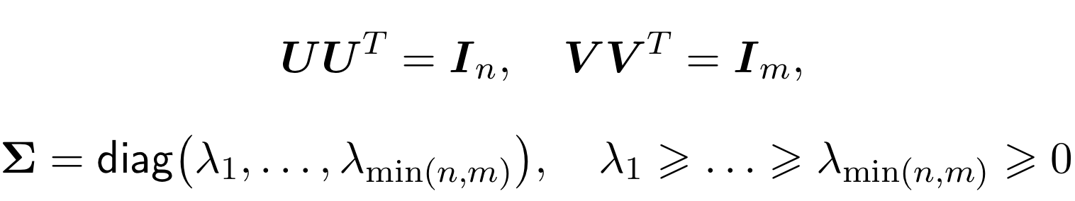
SVD (Singular Value Decomposition), translated as a singular decomposition of the matrix. The singular decomposition theorem states that any matrix 𝐀 of size 𝑛 × 𝑚 has a decomposition into a product of three matrices: 𝑈, Ʃ and 𝑉 𝑇 :
The matrices 𝑈 and 𝑉 are orthogonal, and Ʃ is diagonal (although not square).
Moreover, the lambda in the matrix Ʃ will be ordered by non-increasing. Now we will not prove this theorem, just use the decomposition itself.
But what do we have from the fact that we can some kind of matrix in the product of three even more incomprehensible matrices. For us, the following will be interesting. In addition to the usual decomposition, it is still truncated, when among the lambdas, only the first 𝑑 numbers remain, and the rest we assume to be zero.
This is equivalent to the fact that for matrices 𝑈 and 𝑉 we leave only the first
columns, and the matrix Ʃ is cut to square 𝑑 × 𝑑.
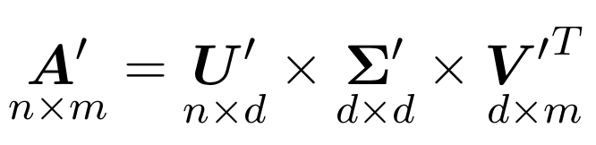
So, it turns out that the obtained matrix 𝐀 ′ well approximates the original matrix 𝐀 and, moreover, is the best low-rank approximation in terms of the standard deviation.
SVD for recommendations
How to use all this for recommendations? We had a matrix, we decomposed it into a product of three matrices. What is not exactly laid out, and approximately. Simplify everything a bit by designating the product of the first two matrices for a single matrix:
Now let's digress a little from all these matrices and concentrate on the resulting algorithm: to predict the user's rating 𝑈 for the movie , we take some vector 𝑝 𝑢 (set of parameters) for this user and vector for this movie 𝑖 . Their scalar product will be the prediction we need: 𝑟̂ 𝑢𝑖 = ⟨𝑝 𝑢 , 𝑞 𝑖⟩ .
The algorithm is quite simple, but it gives surprising results. It does not just allow us to predict estimates. Using it, we can identify hidden signs of objects and user interests by user history. For example, it may happen that at the first coordinate of the vector each user will have a number indicating whether the user looks more like a boy or a girl, the second coordinate is a number reflecting the approximate age of the user. At the same film, the first coordinate will show whether it is more interesting to boys or girls, and the second one - to what age group of users it is interesting.
But not everything is so simple. There are a few problems. First, the estimation matrix is not completely known to us, so we cannot simply take its SVD decomposition. Secondly, the SVD decomposition is not unique: (𝑈Ω) Ʃ (𝑉Ω) = 𝑈Ʃ𝑉 𝑇 , so even if we find at least some decomposition, it is unlikely that the first coordinate in it will correspond to the gender of the user, and the second will be the age.
Training
Let's try to deal with the first problem. Here we need machine learning. So, we cannot find the SVD decomposition of the matrix, since we do not know the matrix itself. But we want to take advantage of this idea and come up with a prediction model that will work in a manner similar to SVD. Our model will depend on many parameters - vectors of users and movies. For the given parameters, in order to predict the estimate, we take the user vector, the vector of the film and get their scalar product:
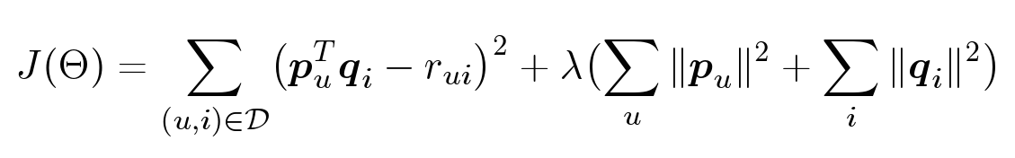
But since we do not know vectors, they still need to be obtained. The idea is that we have user ratings with which we can find the optimal parameters for which our model would predict these ratings as best we can:
So, we want to find such parameters θ so that the error square is as small as possible. But there is a paradox here: we want to make less mistakes in the future , but we do not know what estimates we will ask. Accordingly, we cannot optimize this. But we already know the ratings given by users. Let's try to choose the parameters so that on those estimates that we already have, the error was as small as possible. In addition, we add another term - the regularizer.
Why do we need a regularizer?
Regularization is needed to combat retraining - a phenomenon when the constructed model well explains the examples from the training set, but it does not work well with examples that did not participate in the training. In general, there are several methods to combat retraining; I would like to mention two of them. First, you need to choose simple models. The simpler the model, the better it summarizes the future data (this is similar to the well-known principle of Occam's razor). And the second method is just regularization. When we set up a model for a training set, we optimize the error. Regularization is that we optimize not just an error, but an error plus some function of the parameters (for example, the norm of the vector of parameters). This allows you to limit the size of the parameters in the solution, reduces the degree of freedom of the model.
Numerical optimization
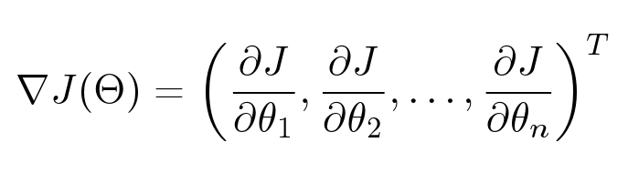
How do we find the optimal parameters? We need to optimize this functionality:
There are many parameters: for each user, for each object we have our own vector, which we want to optimize. We have a function depending on a large number of variables. How to find her minimum? Here we need a gradient - a vector of partial derivatives for each parameter.
Gradient is very convenient to visualize. The illustration shows the surface: a function of two variables. For example, the altitude above sea level. Then the gradient at any particular point is a vector directed in the direction where our function grows the most. And if you run water from this point, it will flow in the direction opposite to the gradient.
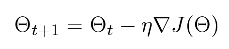
The most well-known method for optimizing functions is gradient descent. Suppose we have a function of many variables, we want to optimize it. We take some initial value, and then we look where we can move in order to minimize this value. The gradient descent method is an iterative algorithm: it repeatedly takes the parameters of a certain point, looks at the gradient and steps against its direction:
The problems with this method lie in the fact that, firstly, in our case, it works very slowly and, secondly, it finds local, rather than global, minima. The second problem is not so terrible for us, because In our case, the value of the functional in local minima is close to the global optimum.
Alternating least squares
However, the gradient descent method is not always necessary. For example, if we need to calculate the minimum for a parabola, there is no need to act by this method, we know for sure where its minimum is. It turns out that the functionality that we are trying to optimize - the sum of the squares of errors plus the sum of the squares of all parameters - is also a quadratic functional, it is very similar to a parabola. For each specific parameter, if we fix all the others, it will be just a parabola. Those. at least one coordinate we can accurately determine. The Alternating Least Squares method is based on this consideration. I will not dwell on it in detail. Let me just say that in it we alternately accurately find minima in one coordinate or another:
We fix all the parameters of the objects, optimize exactly the parameters of the users, further fix the parameters of the users and optimize the parameters of the objects. We act iteratively:
It all works quickly enough, with each step can be parallelized.
Measuring the quality of recommendations
If we want to improve the quality of recommendations, we need to learn how to measure it. For this, an algorithm trained on one sample — a training one — is tested on another - a test one. Netflix suggested measuring the quality of recommendations for the RMSE metric:
Today it is the standard metric for predicting an estimate. However, it has its drawbacks:
- Each user has their own idea of the rating scale. Users who have a wider scatter of ratings will have a greater influence on the value of the metric than others.
- A mistake in predicting a high score has the same weight as a mistake in predicting a low score. At the same time, it is more terrible to predict a rating of 9 instead of a real assessment of 7 than to predict 4 instead of 2 (on a ten-point scale).
- You can have an almost perfect RMSE metric, but have very poor ranking quality, and vice versa.
Ranking metrics
There are other metrics - ranking metrics, for example, based on completeness and accuracy. Let 𝑹 be the set of recommended objects, 𝑷 the set of objects that the user will actually like.
There are also problems here:
- There is no data about the recommended objects that the user has not rated.
- Optimizing these metrics directly is almost impossible.
Other recommendation properties
It turns out that the perception of recommendations is influenced not only by the quality of ranking, but also by some other characteristics. Among them, for example, variety (you should not give the user movies only on one topic or from one series), surprise (if you recommend very popular movies, such recommendations will be too banal and almost useless), novelty (many people like classic films, but recommendations usually used to discover something new) and many others.
Similar objects
Similarity of objects is not such an obvious thing. There are different approaches to this task:
- Similar objects are objects that are similar in their characteristics (content-based).
- Similar objects are objects that are often used together (“customers who bought 𝑖 also bought”).
- Similar objects are recommendations to the user who liked this object.
- Similar objects are simply guidelines in which the object acts as a context.
Development directions
Conceptual issues
- How to build lists of recommendations based on predictions? (Plain top is not always the best idea.)
- How to improve the quality of recommendations, not predictions?
- How to measure the similarity of objects?
- How to justify the recommendations? (It turns out that users perceive recommendations much better if they provide them with some explanations.)
Technical issues
- How to solve the cold start problem for new users and new objects?
- How to quickly update the recommendations? (The benefits of introducing recommendations into your service may depend on this.)
- How to quickly find objects with the highest prediction?
- How to measure the quality of online recommendations? (The traditional approach with training and test samples may not work very well.)
- How to scale the system?
How to consider additional information?
- How to take into account not only explicit , but also implicit feedback? (Implicit feedback is often orders of magnitude greater.)
- How to take into account the context? (Context-aware recommendations)
- How to take into account the signs of objects? (Hybrid systems)
- How to take into account the connection between objects? (taxonomy)
- How to take into account signs and user connections?
- How to account for information from other sources and subject areas? (Cross-domain recommendations)
Literature
- Introduction to Algebra , Kostrikin A.I.
- Mathematical analysis , Zorich V. A.
- Machine learning , Vorontsov KV, lecture course
Source: https://habr.com/ru/post/241455/
All Articles