Mathematical drawings
In this post I will give a few drawings, drawn with the help of mathematical formulas. The purpose of these drawings is not just to draw something on the screen (there is computer graphics for this), but to offer a simple formula that defines the drawing.

The first picture shows a lotus. Figure built in the program Wolfram Mathematica.
These formulas are simpler to present in a spherical coordinate system: the length of the radius vector latitude
  longitude
  . Here is the parameter
  . Its meaning is that we take a point with longitude
  and retreat from it to
  in the direction of decreasing and increasing longitude.
')
The next picture is a pretty flower. The formula is given in a spherical coordinate system, and a compression transformation along the z axis is also done.
Here is another flower.

This figure shows the balls obtained as a surface of revolution for a certain function.
The drawing reminds of the ACM World Programming Championship, the quarter-finals of which are held in the fall. (At the finals of this championship, the team is given a ball for the correctly solved task.)
Now I will give a few holiday drawings.
Here is a drawing made for the New Year. This is a Christmas tree, built with the help of segments.
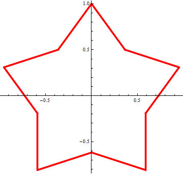
This is a star made on February 23.
The asterisk is given using the polar straight line equation.
By the way, the parameter (half the angle of the star's beam) can vary. This star corresponds to the value
  .
.
With we get a starfish like starfish:
With we get a pointed star:

Here is a picture that fits Valentine's Day.

You can even make a mathematical confession:

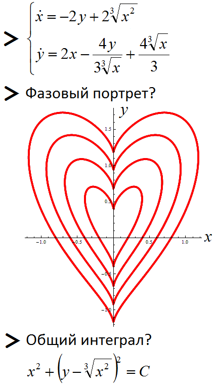
And here is another mathematical heart. An autonomous system of 2 differential equations of the 1st order is considered. A phase portrait of this system was constructed (the trajectories of the system are drawn under different initial conditions) and the general integral of the system is found.
This system can be obtained by differentiating the general integral with respect to t. In this way (solving a system of differential equations) you can build graphs of equations.
And this is a mathematical card for March 8. The figure shows a certain abstract computer that has plotted the Bernoulli lemniscates.

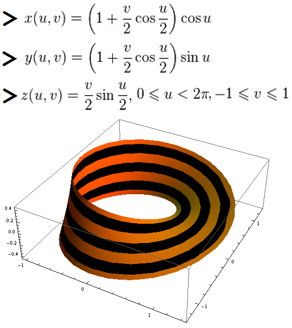
The illustration shows the St. George Mobius Ribbon by May 9.
The following figure shows a square academic cap, the figure is suitable for September 1.

This picture shows the FEFU logo:
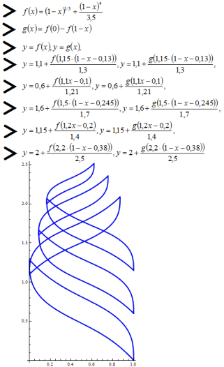
Here is the logo itself:

And this is the three-dimensional FEFU logo, which is also built according to mathematical formulas in the Wolfram Mathematica package.

The first picture shows a lotus. Figure built in the program Wolfram Mathematica.
Code
phi = 0; dphi = 2*Pi/7; theta[r_] := 0.4*r; theta1[r_] := 1*r; theta2[r_] := 0.7*r; Show[ ParametricPlot3D[{r*Cos[phi], r*Sin[phi], 0}, {r, 0, 0.8}, {phi, 0, 2 Pi}, PlotStyle -> Darker[Green], Mesh -> None], ParametricPlot3D[{r*Cos[phi], r*Sin[phi], 0.02}, {r, 0, 0.15}, {phi, 0, 2 Pi}, PlotStyle -> Yellow, Mesh -> None], ParametricPlot3D[ Join[ Table[ {r*Cos[theta[r]]*Cos[(i*dphi) + t*dphi/2*r*(1 - r)^1.5*5], r*Cos[theta[r]]*Sin[(i*dphi) + t*dphi/2*r*(1 - r)^1.5*5], r*Sin[theta[r]]}, {i, 0, 6}], Table[{r*Cos[theta1[r]]*Cos[(i*dphi) + t*dphi/2*r*(1 - r)^1.5*5], r*Cos[theta1[r]]*Sin[(i*dphi) + t*dphi/2*r*(1 - r)^1.5*5], r*Sin[theta1[r]]}, {i, 0, 6}], Table[{r*Cos[theta2[r]]* Cos[(dphi/2 + i*dphi) + t*dphi/2*r*(1 - r)^1.5*5], r*Cos[theta2[r]]* Sin[(dphi/2 + i*dphi) + t*dphi/2*r*(1 - r)^1.5*5], r*Sin[theta2[r]]}, {i, 0, 6}]], {r, 0, 1}, {t, -1, 1}, PlotStyle -> Directive[Specularity[RGBColor[1, 0.3, 0], 20], RGBColor[0.972, 0.658, 0.898], Lighting -> {{"Directional", Darker[White, 0.5], {2, 0, 2}}, {"Ambient", Darker[White]}}], Mesh -> None], PlotRange -> {{-0.85, 0.85}, {-0.85, 0.85}, {0, 0.8}}] These formulas are simpler to present in a spherical coordinate system: the length of the radius vector
latitude longitude . Here is the parameter . Its meaning is that we take a point with longitude and retreat from it to in the direction of decreasing and increasing longitude.')
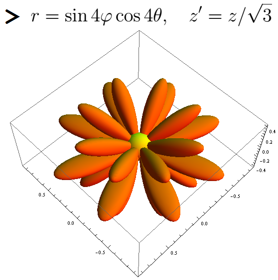
The next picture is a pretty flower. The formula is given in a spherical coordinate system, and a compression transformation along the z axis is also done.
Code
r[theta_, phi_] := If[(Pi/2 - Abs[theta] < Pi/8), 0.25*Sin[theta], Sin[4*phi]*Cos[4*theta]]; Show[ParametricPlot3D[ {r[theta, phi]*Cos[theta]*Cos[phi], r[theta, phi]*Cos[theta]*Sin[phi], r[theta, phi]*Sin[theta]/Sqrt[3]}, {theta, -Pi/2, Pi/2}, {phi, 0, 2*Pi}, Mesh -> None, PlotStyle -> Orange, PlotRange -> All, MaxRecursion -> 4], SphericalPlot3D[0.16, theta, phi, Mesh -> None, PlotStyle -> Yellow]] Here is another flower.
Code
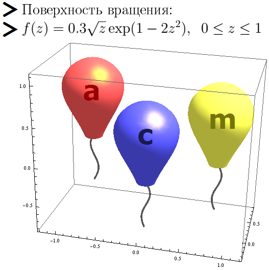
xx[t_] := 0; yy[t_] := -0.75 t*(1 - t); zz[t_] := -3 t; rr = 0.05; x1[t_] := 0; y1[t_] := -0.15 + 0.5 t; z1[t_] := -1.6 + 0.5 t; r[theta_, phi_] := If[(Pi/2 - Abs[theta] < Pi/8), 0.25*Sin[theta], Sin[4*phi]*Cos[4*theta]]; Show[ParametricPlot3D[ {r[theta, phi]*Cos[theta]*Cos[phi], r[theta, phi]*Cos[theta]*Sin[phi], r[theta, phi]*Sin[theta]/Sqrt[3]}, {theta, -Pi/2, Pi/2}, {phi, 0, 2*Pi}, Mesh -> None, PlotStyle -> Orange, PlotRange -> All, MaxRecursion -> 4], SphericalPlot3D[0.16, theta, phi, Mesh -> None, PlotStyle -> Yellow], ParametricPlot3D[{xx[t] + rr*Cos[phi], yy[t] + rr*Sin[phi], zz[t]}, {t, 0, 1}, {phi, 0, 2 Pi}, Mesh -> None, PlotStyle -> Green], ParametricPlot3D[{x1[t] + phi*t*(1 - t), y1[t] - 0.5 phi*t*(1 - t)^3, z1[t]}, {t, 0, 1}, {phi, -1, 1}, Mesh -> None, PlotStyle -> Green], Boxed -> False, Axes -> None] This figure shows the balls obtained as a surface of revolution for a certain function.
Code
x1 = 0; y1 = 0; z1 = -0.2; x2 = 0.8; y2 = 0.3; z2 = 0; x3 = -0.8; y3 = 0.5; z3 = 0.1; f[z_] := z*(1 - z); f[z_] := 0.3 z^0.5*Exp[1 - 2 z^2]; gz[t_] := -0.6 t; gy[t_] := 0.1 t*(1 - t); gx[t_] := 0.05 Sin[6 t]; Show[ParametricPlot3D[{x1 + f[1 - z]*Cos[phi], y1 + f[1 - z]*Sin[phi], z1 + z}, {z, 0, 1}, {phi, 0, 2*Pi}, PlotStyle -> Directive[Specularity[RGBColor[1, 0.8, 0], 30], Lighter[Blue], Lighting -> {{"Directional", White, {1.5, 0, 3}}, {"Ambient", Darker[White]}}], Mesh -> None], ParametricPlot3D[{x1 + gx[t], y1 + gy[t], z1 + gz[t]}, {t, 0, 1}, PlotStyle -> Directive[Thickness[0.0075], Lighter[Black]]], ParametricPlot3D[{x2 + f[1 - z]*Cos[phi], y2 + f[1 - z]*Sin[phi], z2 + z}, {z, 0, 1}, {phi, 0, 2*Pi}, PlotStyle -> Directive[Specularity[RGBColor[1, 0.8, 0], 30], Lighter[Yellow], Lighting -> {{"Directional", White, {1.5, 0, 3}}, {"Ambient", Darker[White]}}], Mesh -> None], ParametricPlot3D[{x3 + f[1 - z]*Cos[phi], y3 + f[1 - z]*Sin[phi], z3 + z}, {z, 0, 1}, {phi, 0, 2*Pi}, PlotStyle -> Directive[Specularity[RGBColor[1, 0.8, 0], 30], Lighter[Red], Lighting -> {{"Directional", White, {1.5, 0, 3}}, {"Ambient", Darker[White]}}], Mesh -> None], ParametricPlot3D[{x2 + gx[1 - t], y2 + gy[1 - t], z2 + gz[1 - t]}, {t, 0, 1}, PlotStyle -> Directive[Thickness[0.0075], Lighter[Black]]], ParametricPlot3D[{x3 + gx[t], y3 + gy[1 - t], z3 + gz[1 - t]}, {t, 0, 1}, PlotStyle -> Directive[Thickness[0.0075], Lighter[Black]]], PlotRange -> All] The drawing reminds of the ACM World Programming Championship, the quarter-finals of which are held in the fall. (At the finals of this championship, the team is given a ball for the correctly solved task.)
Now I will give a few holiday drawings.
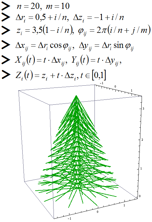
Here is a drawing made for the New Year. This is a Christmas tree, built with the help of segments.
Code
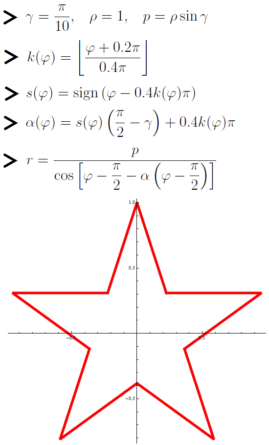
a = 1; b = 0.5; c = 1.5; h = 3.5; dr[k_] := b + (c - b)/n*k; dz[k_] := -(a - a/n*k); z[k_] := h - h*k/n; cnt = 0; Do[Do[cnt = cnt + 1; phi = j*2*Pi/m + i*2*Pi/n; ldx[cnt] = dr[i]*Cos[phi]; ldy[cnt] = dr[i]*Sin[phi]; ldz[cnt] = dz[i]; lz[cnt] = z[i], {j, 1, m}], {i, 1, n}] ParametricPlot3D[ Table[{ldx[i]*t, ldy[i]*t, lz[i] + ldz[i]*t}, {i, 1, cnt}], {t, 0, 1}, PlotStyle -> Directive[Darker[Green], Thickness[0.005]] This is a star made on February 23.
Code
gamma = Pi/10; rho = 1; p = rho*Sin[gamma]; k[phi_] := Floor[(phi + 0.2*Pi)/(0.4*Pi)]; s[phi_] := Sign[phi - 0.4*k[phi]*Pi]; alpha[phi_] := s[phi]*(Pi/2 - gamma) + 0.4*k[phi]*Pi; PolarPlot[p/Cos[phi - Pi/2 - alpha[phi - Pi/2]], {phi, 0, 2*Pi}, PlotStyle -> Directive[Red, Thickness[0.01]]] The asterisk is given using the polar straight line equation.
By the way, the parameter
(half the angle of the star's beam) can vary. This star corresponds to the value .With
we get a starfish like starfish:With
we get a pointed star:Here is a picture that fits Valentine's Day.
Code
f[x_, y_] := x^2 + (y - (x^2)^(1/3))^2 - 1; h1[x_] := (x^2)^(1/3) + Sqrt[1 - x^2]; h2[x_] := (x^2)^(1/3) - Sqrt[1 - x^2]; Do[x0[i] = 1 - (i - 1)/6; y0[i] = h1[x0[i]]; k[i] = 4 + i, {i, 1, 6}]; x0[7] = 0; y0[7] = h1[x0[7]]; k[7] = 7; xx0[1] = 0.95; yy0[1] = h2[xx0[1]]; kk[1] = 6; Do[xx0[i] = 1.1 - 0.15*i; yy0[i] = h2[xx0[i]]; kk[i] = 4 + i, {i, 2, 6}] xx0[7] = 0; yy0[7] = h2[xx0[7]]; kk[7] = 6; RegionPlot[ Or @@ Table[(f[(x - x0[i])*k[i], (y - y0[i])*k[i]] <= 0) || (f[(x + x0[i])*k[i], (y - y0[i])*k[i]] <= 0), {i, 1, 7}] || Or @@ Table[(f[(x - xx0[i])*kk[i], (y - yy0[i])*kk[i]] <= 0) || (f[(x + xx0[i])*kk[i], (y - yy0[i])*kk[i]] <= 0), {i, 1, 7}], {x, -1.5, 1.5}, {y, -2.5, 2.5}, PlotStyle -> Red, AspectRatio -> 0.9, PlotRange -> All, MaxRecursion -> 5] You can even make a mathematical confession:
And here is another mathematical heart. An autonomous system of 2 differential equations of the 1st order is considered. A phase portrait of this system was constructed (the trajectories of the system are drawn under different initial conditions) and the general integral of the system is found.
This system can be obtained by differentiating the general integral with respect to t. In this way (solving a system of differential equations) you can build graphs of equations.
And this is a mathematical card for March 8. The figure shows a certain abstract computer that has plotted the Bernoulli lemniscates.
The illustration shows the St. George Mobius Ribbon by May 9.
Code
f[i_, u_] := If[i == 0, -1 + 1/7 + u/7, If[i == 6, -1 + 2*i/7 + u/7, -1 + 2*i/7 + u*2/7]]; ParametricPlot3D[ Evaluate@Table[{(1 + f[i, u]/2*Cos[phi/2])* Cos[phi], (1 + f[i, u]/2*Cos[phi/2])*Sin[phi], f[i, u]/2*Sin[phi/2]}, {i, 0, 6}], {u, 0, 1}, {phi, 0, 2*Pi}, Mesh -> None, PlotStyle -> {Orange, Black, Orange, Black, Orange, Black, Orange}] The following figure shows a square academic cap, the figure is suitable for September 1.
Code
RegionPlot3D[((x^2 + y^2 + (z + 1.75)^2 <= 4 && x^2 + y^2 + (z + 1.75)^2 >= 4 - 1.4) || (z <= 0.1 && z >= 0)) && (z >= -1.5), {x, -2, 2}, {y, -2, 2}, {z, -2, 0.1}, BoxRatios -> {1, 1, 0.8}, PlotStyle -> Blue] This picture shows the FEFU logo:
Here is the logo itself:
And this is the three-dimensional FEFU logo, which is also built according to mathematical formulas in the Wolfram Mathematica package.
Code
g[z_] := 1/(1 + (1 - z)^2) - 1/2; h[z_] := 1 - 1/2*Sqrt[1 + (z*Sqrt[3])^2]; f[z_] := If[z >= 0 && z <= 1, g[z], If[z >= 1 && z <= 2, h[z - 1]]] phit[t_] := 2*Pi*t; zt[t_] := 1.4*t; zt1[t_] := 0.3 + 1.4*t; zt2[t_] := 0.6 + 1.4*t; phit1[t_] := 2*Pi*t; phit2[t_] := 2*Pi*t; k = 0.111; ParametricPlot3D[{{f[zt[t] + k*s]*Cos[phit[t]], f[zt[t] + k*s]*Sin[phit[t]], zt[t] + k*s}, {f[zt1[t] + k*s]*Cos[phit1[t]], f[zt1[t] + k*s]*Sin[phit1[t]], zt1[t] + k*s}, {f[zt2[t] + k*s]*Cos[phit2[t]], f[zt2[t] + k*s]*Sin[phit2[t]], zt2[t] + k*s}}, {t, 0, 1}, {s, -1, 1}, PlotStyle -> Blue, Mesh -> None, Axes -> False, Boxed -> False] Source: https://habr.com/ru/post/241449/
All Articles