Money, goods and some statistics
A couple of years ago I came across an interesting article about the relationship between the prices of gold and oil.
And I decided to expand the model a little and conduct my own research.
First of all, take not two products, but some more substantial set.
After a long search on the Internet, I found this site from which I downloaded the price archive ( download XLS ) for goods for 35 years.
')
I processed all the data in MATLAB.
As a relative price for more than two products, you can use the price divided by the geometric average:
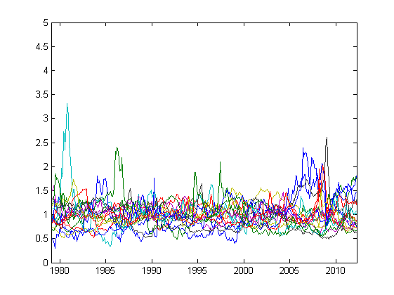
Charts pricing:
Standard deviations of relative prices as a percentage of the average time:
Now we will try to create a diversified product (DP).
Let x be the vector of the relative quantity of goods, sum (x i ) = 1;
A is the covariance matrix of normalized prices.
Then the variance of the diversified product is calculated as X '* A * X;
We need to minimize it.
A typical problem for the conditional extremum is solved by the method of Lagrange multipliers.
I will not go into details, it is solved like this:
The composition of the DP is obtained as follows:
Calculate the cost of DP:
Build graphics:

Above is a relative cost chart, below is a dollar value.
The standard deviation of the relative cost of PD for more than 30 years is only 1.06%!
But its value in dollars has increased (respectively, the purchasing power of the dollar has fallen).
So what might this purchasing power depend on?
Once I came across data on the public debt of the United States.
Here (pp. 143-144) here I found detailed data on public debt and overtook them in the XLS file .
Get the data from the table:
And try to build graphics:
The top chart is the volume of US public debt in millions of dollars, the bottom one is a percentage of GDP.
You can notice some similarities in the behavior of debt in% of GDP and the cost of a diversified product.
So why not try to superimpose these two graphs on each other?
To do this, smooth the cost of the PD with the moving average, and interpolate the amount of debt over the entire time interval, and also divide by the time average:
We get the following picture:
You can also calculate the correlation coefficient between the value of the PD in dollars and the amount of debt, it is equal to 0.7165 or 71.65% - the figure is quite significant.
Fully matlab-script can be viewed on github (link updated 09/06/2017).
How is the economy today?
As is known, most international transactions are made in US dollars.
The ruble is also pegged to the dollar - the Central Bank can issue exactly as many rubles to the economy as dollars received from exports, multiplying this amount by the dollar / ruble rate.
What can be done?
Introduce the concept of a balanced currency unit (ETS) and link it not to a certain foreign currency, but to a diversified product.
You can implement it like this:
Suppose there is an ETS and a currency of some foreign state V.
The ETS rate in relation to V is indexed as the value of the PD in currency V, multiplied by a certain coefficient q.
Consider export and import operations.
Suppose 1V = 20 Cde.
Export.
Option 1.
An external buyer purchases goods in the amount of 1000V or 20000CEE in currency V.
1000V "settles" in the Central Bank, 20000CEU is emitted into the economy.
Option 2.
An external buyer borrows from the Central Bank 20000CEU and buys goods for them.
That is, in fact, undertakes to return an equal amount of goods in the future.
Import.
Option 1.
Domestic buyer purchases from the outside goods in the amount of 1000V or 20000CEE in currency V.
The Central Bank issues 1000V from its reserves, 20000 ETSE is withdrawn from the economy.
Option 2.
An internal buyer purchases from outside the goods in the ETS.
Conclusion: the introduction of ETS in theory allows virtually to avoid inflation and to introduce interest rates on loans close to zero.
And I decided to expand the model a little and conduct my own research.
First of all, take not two products, but some more substantial set.
After a long search on the Internet, I found this site from which I downloaded the price archive ( download XLS ) for goods for 35 years.
')
I processed all the data in MATLAB.
xls = xlsread('data.xls'); % XLS time = 1:399; % real_time = 1979 + time/12; % data = xls(time,1:22); % : oil = data(:,1); % gold = data(:,2); % iron = data(:,3); % logs = data(:,4); % maize = data(:,5); % beef = data(:,6); % % % , : all_goods = [oil gold logs maize beef chicken gas tea tobacco wheat sugar soy rice cotton copper coffee coal]; goods_count = size(all_goods, 2); % As a relative price for more than two products, you can use the price divided by the geometric average:
geom_average = ones(size(time))'; % ' %, for i = 1:goods_count geom_average = geom_average .* all_goods(:,i); end geom_average = geom_average .^ (1/goods_count); % all_goods_rel = zeros(size(all_goods)); all_goods_norm = zeros(size(all_goods)); mean_ = zeros(1,goods_count); std_ = zeros(1,goods_count); percent_std_ = zeros(1,goods_count); for i = 1:goods_count all_goods_rel(:,i) = all_goods(:,i) ./ geom_average; % mean_(i) = mean(all_goods_rel(:,i)); % all_goods_norm(:,i) = all_goods_rel(:,i) / mean_(i); % , std_(i) = std(all_goods_rel(:,i)); % percent_std_(i) = 100*std_(i)/mean_(i); % end Charts pricing:
Standard deviations of relative prices as a percentage of the average time:
| Raw oil | 37.77% | Gas | 32.18% | Pic | 19.71% |
| Gold | 21.57% | Tea | 25.18% | Cotton | 24.52% |
| Log | 20.33% | Tobacco | 20.55% | Copper | 36.24% |
| Corn | 15.71% | Wheat | 14.58% | Coffee | 37.08% |
| Beef | 19.39% | Sugar | 37.91% | Coal | 21.68% |
| Chicken meat | 25.47% | Soy | 12.68% |
Now we will try to create a diversified product (DP).
Let x be the vector of the relative quantity of goods, sum (x i ) = 1;
A is the covariance matrix of normalized prices.
Then the variance of the diversified product is calculated as X '* A * X;
We need to minimize it.
A typical problem for the conditional extremum is solved by the method of Lagrange multipliers.
I will not go into details, it is solved like this:
A = cov(all_goods_rel); % cond = ones(1, goods_count); B = [2*A cond']; %' B = [B; [cond 0]]; b = [zeros(1, goods_count) 1]'; x = (B^-1)*b; The composition of the DP is obtained as follows:
| Raw oil | 0,0035 barrels | Gas | 23.2 thousand BTU | Pic | 310.3 g |
| Gold | 9.627 mg | Tea | 76.3 g | Cotton | 98.1 g |
| Log | 0.353 cc dm | Tobacco | 45.69 g | Copper | 45.79 g |
| Corn | 970.2 g | Wheat | 514.2 g | Coffee | 40.7 g |
| Beef | 64.2 g | Sugar | 538.8 g | Coal | 3.5 kg |
| Chicken meat | 148.8 g | Soy | 416.5 g |
Calculate the cost of DP:
DP = all_goods_rel*x(1:goods_count); % USD_per_DP = all_goods*x(1:goods_count); % Build graphics:
Above is a relative cost chart, below is a dollar value.
The standard deviation of the relative cost of PD for more than 30 years is only 1.06%!
But its value in dollars has increased (respectively, the purchasing power of the dollar has fallen).
So what might this purchasing power depend on?
Once I came across data on the public debt of the United States.
Get the data from the table:
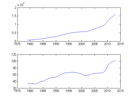
debt_xls = xlsread('usa_debt.xls'); debt_time = debt_xls(:,1); end_index = size(debt_time,1); start_index = (1:end_index)*(debt_time == 1978); debt_time = debt_time(start_index:end_index); debt_usd = debt_xls(start_index:end_index,2); debt_percent = debt_xls(start_index:end_index,3); debt_time = debt_time + 1; % , And try to build graphics:
The top chart is the volume of US public debt in millions of dollars, the bottom one is a percentage of GDP.
You can notice some similarities in the behavior of debt in% of GDP and the cost of a diversified product.
So why not try to superimpose these two graphs on each other?
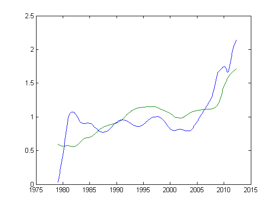
To do this, smooth the cost of the PD with the moving average, and interpolate the amount of debt over the entire time interval, and also divide by the time average:
a = 1; b = ones(1,24)/24; debt_interp = interp1(debt_time, debt_percent, real_time, 'cubic')'; %' USD_per_DP_mov_av = filter(b, a, USD_per_DP); debt_and_DP = [USD_per_DP_mov_av/mean(USD_per_DP_mov_av) debt_interp/mean(debt_interp)]; debt_DP_corr = corr2(debt_and_DP(:,1),debt_and_DP(:,2)) figure; plot(real_time, debt_and_DP); We get the following picture:
You can also calculate the correlation coefficient between the value of the PD in dollars and the amount of debt, it is equal to 0.7165 or 71.65% - the figure is quite significant.
Fully matlab-script can be viewed on github (link updated 09/06/2017).
Afterword
How is the economy today?
As is known, most international transactions are made in US dollars.
The ruble is also pegged to the dollar - the Central Bank can issue exactly as many rubles to the economy as dollars received from exports, multiplying this amount by the dollar / ruble rate.
What can be done?
Introduce the concept of a balanced currency unit (ETS) and link it not to a certain foreign currency, but to a diversified product.
You can implement it like this:
Suppose there is an ETS and a currency of some foreign state V.
The ETS rate in relation to V is indexed as the value of the PD in currency V, multiplied by a certain coefficient q.
Consider export and import operations.
Suppose 1V = 20 Cde.
Export.
Option 1.
An external buyer purchases goods in the amount of 1000V or 20000CEE in currency V.
1000V "settles" in the Central Bank, 20000CEU is emitted into the economy.
Option 2.
An external buyer borrows from the Central Bank 20000CEU and buys goods for them.
That is, in fact, undertakes to return an equal amount of goods in the future.
Import.
Option 1.
Domestic buyer purchases from the outside goods in the amount of 1000V or 20000CEE in currency V.
The Central Bank issues 1000V from its reserves, 20000 ETSE is withdrawn from the economy.
Option 2.
An internal buyer purchases from outside the goods in the ETS.
Conclusion: the introduction of ETS in theory allows virtually to avoid inflation and to introduce interest rates on loans close to zero.
Source: https://habr.com/ru/post/240145/
All Articles