Such a different Blur

I'll tell you about the different implementations of the blur effect on GLSL.

To begin with, I want to warn you right away - I have set restrictions for myself to use the GLSL version no higher than 1.1. This is necessary in order for the application to work on as many devices and systems as possible. So, for example, I had at my disposal an iMac with a Radeon HD 6750M and the most supported version of GLSL 1.2, a laptop with Kubuntu on intel hd 4000 with version GLSL 1.3 and a desktop with GeForce gtx560.
I will try to describe the effects in simple words and without complicated formulas, the main goal is to give examples of blurring methods. The article is a preparatory to the next two articles.

Gaussian blur

Consider the classic Gaussian blur. Where just about him was not written, perhaps this is the most popular way to blur gamedev and not only. But I can not not consider it, at least in brief.
What is a blur in general? Roughly speaking, this is the averaging of neighboring pixels, that is, considering the current pixel, we find the average color of all its neighbors in a certain radius. But if you use a simple arithmetic average (uniform distribution), then the blur will not be very beautiful. Therefore, it is common to multiply neighbors by coefficients, the values of which obey the normal distribution law (it is the Gauss distribution, hence the name blur).
')

blur with a uniform and normal distribution, respectively

Gaussian blur has one important property - separability. This makes it possible to divide the algorithm into two parts - a blur along the x coordinate and a blur along y. Thus, the coefficients do not need to be calculated for all neighbors, it suffices to find for one column or row. The coefficients can be found by the Gauss formula:

,
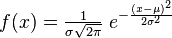where μ is the mathematical expectation, and σ is the variance.

The implementation of such a blur is quite simple, we need two buffers of the same format and a pre-calculated array of blur coefficients:

Render the scene to the first buffer
Render the image to the second buffer with a vertical shading blur
Render again to the first horizontal blur

Shaders

Vertex:

#version 110 attribute vec2 vertex; attribute vec2 texCoord; varying vec2 vTexCoord; void main() { gl_Position = vec4(vertex, 0.0, 1.0); vTexCoord = texCoord; }

Fragment:

 #version 110 const int MAX_KOEFF_SIZE = 32; //   ( ) uniform sampler2D texture; //  uniform int kSize; //  uniform float koeff[MAX_KOEFF_SIZE]; // uniform vec2 direction; //       aspect ratio,  (0.003, 0.0) -   (0.0, 0.002) -  varying vec2 vTexCoord; //    void main() { vec4 sum = vec4(0.0); //  vec2 startDir = -0.5*direction*float(kSize-1); //    for (int i=0; i<kSize; i++) //    sum += texture2D(texture, vTexCoord + startDir + direction*float(i)) * koeff[i]; //  gl_FragColor = sum; }

Bokeh effect

Actually, this is the main reason for writing this article - I wanted to tell you how easy it is to get this effect . The algorithm is similar to the previous one, but there are differences:

The normal distribution law can be replaced by a uniform
Another third pass is added.
Blur now occurs not vertically and horizontally, but along three vectors, the angle between which is 120 °
In addition to the amount of color, the shader also contains the maximum color for all samples, after which both colors are mixed in a given proportion

Shader

Vertex remains the same, fragmentary:

 #version 110 uniform sampler2D texture; //  uniform vec2 direction; // ,   : (0, 1), (0.866/aspect, 0.5), (0.866/aspect, -0.5),          uniform float samples; // , float -        uniform float bokeh; //   [0..1] varying vec2 vTexCoord; //    void main() { vec4 sum = vec4(0.0); //  vec4 msum = vec4(0.0); //    float delta = 1.0/samples; //     float di = 1.0/(samples-1.0); //  for (float i=-0.5; i<0.501; i+=di) { vec4 color = texture2D(texture, vTexCoord + direction * i); //     sum += color * delta; //  msum = max(color, msum); //    } gl_FragColor = mix(sum, msum, bokeh); //        }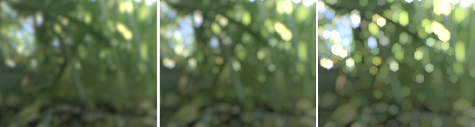

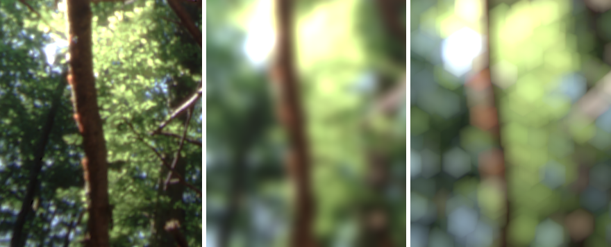
blur with different bokeh ratio: 0.2, 0.5, 0.8 (the image is clickable)

Experimentally, I found out that the best mixing ratio, providing a more or less beautiful effect close to the real one, is 0.5.
Disadvantages of this method:

One draw call has more and about a third more samples than the previous method.
Bokeh shape - only regular polygons with an even number of angles
Cannot be applied in the blur depth algorithm.

There are several other ways to make this effect, here's one of them: we pass through the texture with a special shader, in which we reveal the most contrasting places and write their coordinates into the buffer, then blur the texture in any way without the bokeh effect, after which we render the sprites directly on top of it in the coordinates found in the first step. The advantages of this method - the shape of the bokeh can be of any shape, of the drawbacks - we need geometric shaders, which eliminates weak devices, and you can’t draw on each pixel of the bokeh - we get a wild fill rate.

Depth Blur

The full name of the effect is the depth of the sharply depicted space, or DoF (Depth Of Field). The name speaks for itself - everything that is in focus - clearly, out of focus - is blurry. At first glance, the effect seems simple, but there are moments that complicate it both in terms of the cost of resources and in terms of implementation. One of its drawbacks is that it is impossible to apply previous approaches, due to the fact that it does not have the property of separability, and therefore it cannot be divided into several passes (blurring vertically and horizontally). Sometimes you can cheat: first render the background and blur it, then front without blur. Of course it will not be a full effect, but there will be a feeling of blur in depth. But if the scene is filled with objects across the depth, you will have to blur it in a more “honest” way. But completely honest methods are usually not used - there are too many samples, therefore, as a rule, a small cloud of points is taken as samples within a certain radius from the considered one. The most optimal distribution of such points is called the Poisson disk - it is distinguished from the completely random distribution of points by the fact that the points are approximately equal distance from each other. There are many ways to get a Poisson disk, I use this one for myself:

let r be the radius of the disk, then the upper boundary of the disk is yMax = r, and the lower limit is yMin = -r.
in the yR loop from yMin to yMax, do the following:
find xMax = cos (asin (yR / r)) * r and xMin = -xMax.
in a nested loop with xR from xMin to xMax, we find a point with coordinates (xR, yR).
then we will shift the coordinates of this point by a random variable from -r / 4 to r / 4
the points thus obtained are the sought ones.

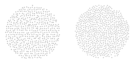
What is this algorithm? We simply roughly divide the circle with a grid and go line by line along the nodes of this grid from left to right from top to bottom. The coordinates of these nodes are randomly slightly shifted and we get the desired Poisson disk.
In fact, this is not exactly a Poisson disk, but it is very similar to it, compare yourself (on the left is my implementation, on the right is the points generated by this algorithm)

C ++ implementation

 float yMax = r; float yMin = -r; yMin += fmod(yMax-yMin, 1)/2; for (float y=yMin; y<yMax; y++) { float xMax = cos(asin(y/r))*r; float xMin = -xMax; xMin += fmod(xMax-xMin, 1)/2; for (float x=xMin; x<xMax; x++) points.append(QPoint(x+floatRand(-r/4, r/4), y+floatRand(-r/4, r/4))); }

There are a lot of points in the pictures above, in fact, about 10-20 are enough. Once the points are obtained, they can be sampled. But first, let's talk about the power of blur.
Information about the strength of the blur for each pixel will be stored in the alpha channel. The strength of the blur varies from -1 to 1, where one is the maximum blur, zero - no blur. I used HDR texture (RGBA16F), but this information can be encoded into an ordinary 8-bit alpha channel:

a = depth * 0.5 + 0.5 - coding
a = depth * 2.0-1.0 - decoding, where depth is the blur power [-1..1]

The depth parameter (blur power) can be calculated using the formula: (focalDistance + zPos) / focalRange, where focalDistance is the focal length, focalRange is the range or depth of the blur. Negativeness of the depth value indicates that the current object or fragment is in front of the focus, if depth is positive, then it is beyond the focus. By the way, in fact, it is not necessary to store a sign, it will double the range of values (it can be critical for an 8-bit texture), but it will be impossible to understand in the shader if there is a fragment in front of or behind the focus - because of this artifacts may occur.

So, by making a sample using the Poisson disc, we get information about the color of the pixel and how hard it is to blur it. Remember the sample rates in the two previous algorithms? So, now in the role of these coefficients is the power of blurring (of course modulo). The blur power also affects the blur radius of the current fragment. You should also talk about the parasitic effect arising in the current implementation - if the depth limit is sharp (transition between far and near objects), then something like a moiré or halo can be observed between them, in this case we simply adjust the coefficient.

As an additional improvement of the algorithm, you can use the second texture - smaller and slightly blurred. This will reduce the number of samples and improve the quality of the blur.

Thanks Chaos_Optima , I forgot to write about the lack of this method: it appears on the borders of nearby objects, when they begin to blur, their borders remain sharp.

Shader

In a fragmentary scene render shader:

 float blur = clamp((focalDistance+zPos)/focalRange, -1.0, 1.0); gl_FragColor = vec4(color, blur);

The vertex blur shader is the same as in the previous methods, fragmentary:

 #version 110 const int MAX_OFFSET_SIZE = 128; //      uniform sampler2D texture; //     uniform sampler2D lowTexture; //       uniform int offsetSize; //      uniform vec2 offsets[MAX_OFFSET_SIZE]; //   varying vec2 vTexCoord; //    void main() { float currentSize = texture2D(texture, vTexCoord).a; //    vec4 resulColor = vec4 (0.0); //  for (int i=0; i<offsetSize; i++) { vec4 highSample = texture2D(texture, vTexCoord+offsets[i]*currentSize); //  vec4 lowSample = texture2D(lowTexture, vTexCoord+offsets[i]*currentSize); float sampleSize = abs(highSample.a);//     highSample.rgb = mix(highSample.rgb, lowSample.rgb, sampleSize); //          highSample.a = highSample.a >= currentSize ? 1.0 : highSample.a; //  (,       ) sampleSize = abs(highSample.a); resultColor.rgb += highSample.rgb * sampleSize; //  resultColor.a += sampleSize; //   } gl_FragColor = resultColor/resultColor.a; }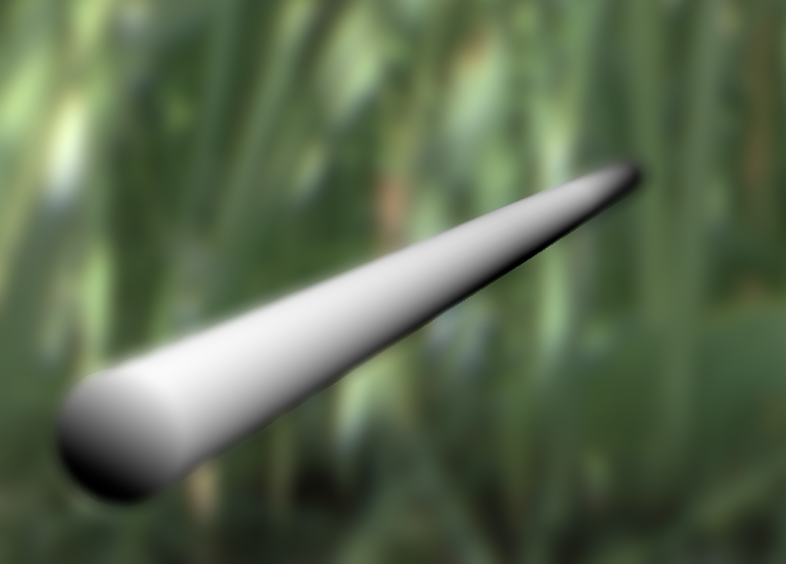

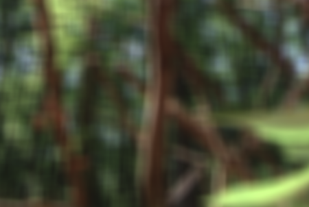
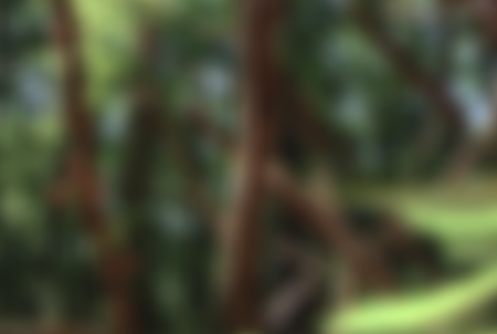
the result of the shader is a blurry stick

Such a different Blur

Gaussian blur

Bokeh effect

Depth Blur

Links

More articles: